Strong Economic Events Indicator (mtbr)This indicator is designed to help traders anticipate market reactions to key economic events and visualize trade levels directly on their TradingView charts. It is highly customizable, allowing precise planning for entries, take-profits, and stop-losses.
Key Features:
Multi-Event Support:
Supports dozens of economic events including ISM Services PMI, CPI, Core CPI, PPI, Non-Farm Payrolls, Unemployment Rate, Retail Sales, GDP, and major central bank rate decisions (Fed, ECB, BOE, BOJ, Australia, Brazil, Canada, China).
Custom Event Date and Time:
Manually set the year, month, day, hour, and minute of the event to match your chart and timezone, ensuring accurate alignment.
Forecast vs Actual Analysis:
Input the forecast and actual values. The indicator calculates the likely market direction (Buy/Sell/Neutral) according to historical market reactions for each event.
Dynamic Trade Levels:
Automatically plots:
Entry price
TP1, TP2, TP3 in pips relative to the entry
Stop Loss in pips relative to the entry
Levels are automatically adjusted based on the event's Buy/Sell direction.
Visual Chart Representation:
Entry: Blue line and label
TP1/TP2/TP3: Green lines and labels
Stop Loss: Red line and label
Event occurrence: Orange dashed vertical line
Informative Table Panel:
Displays at the bottom-right of the chart:
Event name
Entry price
TP1, TP2, TP3 values
Current market direction (Buy/Sell/Neutral)
Customizable Line Extension:
Extend the lines for visibility across multiple bars on the chart.
How to Use the Indicator:
Select the Asset:
Set the Asset to Trade input to the symbol you want to analyze (e.g., XAUUSD, EURUSD).
Choose the Economic Event:
Use the drop-down menu to select the event you want to track.
Set the Event Date and Time:
Input the year, month, day, hour, and minute of the event. This ensures the event lines and labels appear at the correct time on your chart.
Input Forecast and Actual Values:
Enter the forecasted value and the actual result of the event. The script will determine market direction based on historically observed reactions for that event.
Configure Entry and Pip Levels:
Set your Entry Price
Set pip distances for TP1, TP2, TP3, and Stop Loss
The script automatically adjusts the levels according to Buy or Sell direction.
View Levels and Status:
Once the event occurs (or on backtesting), the indicator will plot:
Entry, Take Profits, Stop Loss on the chart
Vertical line for event occurrence
Table summarizing levels and Buy/Sell status
Adjust Line Extension:
Use the Line Extension (bars) input to control how far the horizontal levels extend on the chart.
Example Scenario:
Event: PPI MoM
Forecast: 0.2
Actual: 0.9
The indicator identifies the correct market reaction (Sell for EURUSD) and plots the Entry, TP1, TP2, TP3, and Stop Loss accordingly.
Important Notes:
The indicator does not execute trades automatically; it is for analysis and visualization only.
Always combine the signals with your own risk management and analysis.
Ensure your chart is set to the correct timezone corresponding to the event’s time.
This description fully explains how to use the indicator, what it displays, and step-by-step guidance for beginners and experienced traders
Search in scripts for "stop loss"

Institutional Analyst LLM📊 Institutional Analyst Board LLM – Smart Money Confluence Scanner for XAUUSD, Forex, Crypto 🔍 Overview The Institutional Analyst Board is a complete multi-timeframe smart money toolkit designed for traders who demand clarity, confluence, and precision. It brings together institutional-grade metrics—Order Blocks (OB), Fair Value Gaps (FVG), Liquidity Sweeps, MACD/RSI...
PTS Ultimate Analysis Board (Flexible Position + Ticker)
GoldenTradeClub
GoldenTradeClub
Updated
Jul 15
PTS Ultimate Analysis Board (Flexible Position + Ticker) Version: Pine v5 Description: This indicator builds a fully customizable, multi-timeframe dashboard table that surfaces 19 key metrics for any ticker (current chart TF, 1 h, 4 h). You can position the table at the top-right or bottom-right of your chart and toggle each metric on or off. Key...
Trading Engine AI Light
GoldenTradeClub
GoldenTradeClub
Jul 14
The Trading Engine includes the best and most effective technical analysis tools. It has 27 different Buy Signal parameters and 26 different Sell Signal parameters. Furthermore, it also has 9 Stop Loss triggers for Long Positions and 8 Stop Loss triggers for Short Positions. Many of the Buy or Sell Signal parameters function as Take Profit and Stop Loss signals...
Elliott Wave Complete
GoldenTradeClub
GoldenTradeClub
Jul 4
1. Indicator Presentation Name: Elliott Wave Complete Type: Pine Script v5 overlay dashboard for TradingView Purpose: Automates Elliott Wave motive (1-5) and corrective (A-B-C) pattern detection on any timeframe, enriches it with classic ZigZag pivots, dynamic Fibonacci projection levels, optional wave-count info box, and real-time alerts—all in one...
💀⚡ PTS WIZARD 666™ ULTIMATE SUPREME V5.0 - COMPLETE FIXED ⚡💀
GoldenTradeClub
GoldenTradeClub
Jul 4
1. Indicator Presentation Name: 💀⚡ PTS WIZARD 666™ ULTIMATE SUPREME V5.0 – COMPLETE FIXED Short ID: PTS-666-SUPREME Type: Pine Script v5 overlay dashboard for TradingView Purpose: An all-in-one trading overlay that integrates advanced WaveTrend momentum, RSI/MFI analysis, POC volume profiling, multiple Fibonacci golden/ultimate zones, volume footprint & imbalance...
🔥 PTS TRADE 666™ ULTIMATE BOOKMAP + QUANTUM ENGINE
GoldenTradeClub
GoldenTradeClub
Jul 4
1. Indicator Presentation Name: 🔥 PTS TRADE 666™ ULTIMATE BOOKMAP + QUANTUM ENGINE Short ID: PTS666_QUANTUM_FINAL Type: Pine Script v5 overlay dashboard for TradingView Purpose: A cutting-edge, institutional-grade suite that unifies bookmap-style footprint volume profiling, dynamic heatmap liquidity analysis, AI-driven pattern recognition, smart-money protocols,...
🔥 PTS TRADE 666™ - ULTIMATE INSTITUTIONAL TOOL 🔥
GoldenTradeClub
GoldenTradeClub
Jul 4
1. Indicator Presentation Name: 🔥 PTS TRADE 666™ – ULTIMATE INSTITUTIONAL TOOL V2.0 Short ID: PTS666_UIT_V2 Type: Pine Script v5 overlay dashboard for TradingView Purpose: Combines institutional-grade footprint volume analysis, smart-money structure detection, statistical anomaly checks, multi-timeframe divergence, Ichimoku insights, pattern recognition, and an...
PTS Wizard
GoldenTradeClub
GoldenTradeClub
Jul 4
1. Indicator Presentation Name: PTS Wizard Short Title: PTS Wizard Type: Pine Script v5 overlay dashboard for TradingView Purpose: A unified multi-strategy toolkit that overlays key market insights—liquidity zones, smart-money structure, footprint-style volume profile, consolidation ranges, statistical deviation bands, price forecasts, and session analysis—into a...
🔥 PTS.TRADE 666™ ULTIMATE HYBRID + MTF V3
GoldenTradeClub
GoldenTradeClub
Jul 4
1. Indicator Presentation Name: 🔥 PTS.TRADE 666™ ULTIMATE HYBRID + MTF V3 Short ID: PTS666_ULTIMATE_MTF_V3 Type: Overlay dashboard for TradingView Purpose: A next-level hybrid trading suite that merges institutional-grade order-flow analysis, smart-money concepts, AI-driven insights, classic momentum oscillators (WaveTrend, divergence, “Gold” signals),...
🧙♂ PTS WIZARD V3.0 - FINAL EDITION
GoldenTradeClub
GoldenTradeClub
Jul 4
1. Indicator Presentation Name: 🧙♂ PTS WIZARD V3.0 – FINAL EDITION Short Title: PTS-WIZARD-V3-FINAL Type: Overlay trading dashboard for TradingView Purpose: A comprehensive multi-module indicator that blends classic cipher momentum signals, Elliott Wave pattern detection, advanced statistical analyses (Z-Score, Benford’s Law, Ehlers SNR), footprint-style volume...
🧙♂ PTS WIZARD V3.0 + FOOTPRINT ULTIMATE
GoldenTradeClub
GoldenTradeClub
Jul 4
Name: PTS WIZARD V3.0 + FOOTPRINT ULTIMATE Type: Overlay trading dashboard for TradingView Purpose: Combines classic cipher-style momentum signals with an advanced footprint volume profile, multi-timeframe bias, statistical filters, and a fusion-score system—displayed in a customizable on-chart dashboard. Core Modules Cipher Momentum Signals WaveTrend...
🧙♂ PTS WIZARD V3.0 - BASIC
GoldenTradeClub
GoldenTradeClub
Jul 1
PTS WIZARD V3.0 Basic – Ultimate Multi-Tool Trading Dashboard An all-in-one overlay combining classic cipher signals, Elliott Wave pattern detection, volume analytics, divergence spotting, and smart-entry timing—backed by advanced statistical filters and a live dashboard. Key Features Cipher Signals WaveTrend with overbought/oversold zones & cross signals RSI...
Trading Engine vCD AI
GoldenTradeClub
GoldenTradeClub
Jun 15
The Trading Engine includes the best and most effective technical analysis tools. It has 27 different Buy Signal parameters and 26 different Sell Signal parameters. Furthermore, it also has 9 Stop Loss triggers for Long Positions and 8 Stop Loss triggers for Short Positions. Many of the Buy or Sell Signal parameters function as Take Profit and Stop Loss signals...
Trading Engine vCD
GoldenTradeClub
GoldenTradeClub
Updated
Mar 21
The Trading Engine includes the best and most effective technical analysis tools. It has 27 different Buy Signal parameters and 26 different Sell Signal parameters. Furthermore, it also has 9 Stop Loss triggers for Long Positions and 8 Stop Loss triggers for Short Positions. Many of the Buy or Sell Signal parameters function as Take Profit and Stop Loss signals...
TE CLIENT v13
GoldenTradeClub
GoldenTradeClub
Updated
Mar 15
The Trading Engine includes the best and most effective technical analysis tools. It has 27 different Buy Signal parameters and 26 different Sell Signal parameters. Furthermore, it also has 9 Stop Loss triggers for Long Positions and 8 Stop Loss triggers for Short Positions. Many of the Buy or Sell Signal parameters function as Take Profit and Stop Loss signals...
Trading Engine v13
GoldenTradeClub
GoldenTradeClub
Updated
Mar 15
The Trading Engine includes the best and most effective technical analysis tools. It has 27 different Buy Signal parameters and 26 different Sell Signal parameters. Furthermore, it also has 9 Stop Loss triggers for Long Positions and 8 Stop Loss triggers for Short Positions. Many of the Buy or Sell Signal parameters function as Take Profit and Stop Loss signals...
Trading Engine B2B
GoldenTradeClub
GoldenTradeClub
Updated
Jan 14
The Trading Engine includes the best and most effective technical analysis tools. It has 25 different Buy Signal parameters and 24 different Sell Signal parameters. Furthermore, it also has 9 Stop Loss triggers for Long Positions and 8 Stop Loss triggers for Short Positions. Many of the Buy or Sell Signal parameters function as Take Profit and Stop Loss signals...
Trading Engine B2B FX V9
GoldenTradeClub
GoldenTradeClub
Updated
Jan 14
The VFLOW Trading Engine includes the best and most effective technical analysis tools. It has 20 different Buy Signal parameters and 18 different Sell Signal parameters. Furthermore, it also has 7 Stop Loss triggers for Long Positions and 5 Stop Loss triggers for Short Positions. Many of the Buy or Sell Signal parameters function as Take Profit and Stop Loss...
English
Select market data provided by ICE Data services.
Select reference data provided by FactSet. Copyright © 2025 FactSet Research Systems Inc.
© 2025 TradingView, Inc.
More than a product
Supercharts
Screeners
Stocks
ETFs
Bonds
Crypto coins
CEX pairs
DEX pairs
Pine
Heatmaps
Stocks
ETFs
Crypto
Calendars
Economic
Earnings
Dividends
More products
Yield Curves
Options
News Flow
Pine Script®
Apps
Mobile
Desktop
Tools & subscriptions
Features
Pricing
Market data
Trading
Overview
Brokers
Special offers
CME Group futures
Eurex futures
US stocks bundle
About company
Who we are
Athletes
Blog
Careers
Media kit
Merch
TradingView store
Tarot cards for traders
The C63 TradeTime
Policies & security
Terms of Use
Disclaimer
Privacy Policy
Cookies Policy
Accessibility Statement
Security tips
Bug Bounty program
Status page
Community
Social network
Wall of Love
Refer a friend
House Rules
Moderators
Ideas
Trading
Education
Editors' picks
Pine Script
Indicators & strategies
Wizards
Freelancers
Business solutions
Widgets
Charting libraries
Lightweight Charts™
Advanced Charts
Trading Platform
Growth opportunities
Advertising
Brokerage integration
Partner program
Education program
Look First
Close
Updated 3 hours ago
Institutional Analyst Board
Manage access
Remove from favorites
Use on chart
0
11
Jul 19
📊 Institutional Analyst Board – Smart Money Confluence Scanner for XAUUSD, Forex, Crypto
🔍 Overview
The Institutional Analyst Board is a complete multi-timeframe smart money toolkit designed for traders who demand clarity, confluence, and precision. It brings together institutional-grade metrics—Order Blocks (OB), Fair Value Gaps (FVG), Liquidity Sweeps, MACD/RSI bias, VWAP positioning, and Break of Structure (BoS)—into a single powerful visual dashboard.
This indicator is especially optimized for Gold (XAUUSD) but is also compatible with Crypto and Forex assets.
🧠 Key Features
✅ Multi-Timeframe Dashboard (5M / 15M / 1H)
✅ Order Block Detection with dynamic zones that extend until broken
✅ Fair Value Gap Detection with clear zone shading and border distinction
✅ MACD + RSI Confluence for momentum and bias alignment
✅ VWAP Positioning to identify premium/discount zones
✅ Liquidity Sweeps (internal/external range breaks)
✅ Killzone Highlighting (Asia / London / New York)
✅ Break of Structure (BoS) with advanced confluence filters
✅ Gold Bias Flags across timeframes (BUY / SELL / NEUTRAL)
✅ Dynamic Price Watermark with real-time data
✅ Fully customizable colors, transparencies, and text labels
🧠 How It Works
The Board uses institutional logic to analyze the chart in real time:
Metric Purpose
OB Zones Highlight potential smart money footprints where price is likely to react.
FVG Zones Identify imbalance areas between buyers and sellers—ideal for mean reversion entries.
MACD/RSI Confirm momentum direction and relative strength confluence.
VWAP Determine whether price is trading at a premium or discount.
Liquidity Sweeps Detect manipulative moves before major reversals.
BoS Mark potential trend reversals, filtered by institutional confluence.
Each signal is computed across 3 timeframes and visualized in a clean board that updates live. You’ll also see labels, alerts, and session overlays for maximum clarity.
📌 Ideal Use Case
This tool is perfect for:
Funded Challenge Traders (FTMO, MyForexFunds, etc.)
Gold scalpers and intraday traders
Crypto price action traders using BTC, ETH, SOL, etc.
Smart Money Concept (SMC) and ICT followers
⚙️ Customization Options
Toggle each module (OB, FVG, VWAP, MACD/RSI, etc.)
Set transparency and color for each zone type
Adjust Killzone timing (Asia, London, NY)
Control board position (Top/Bottom) and metric visibility
📈 Compatible Assets
✅ XAUUSD (optimized)
✅ Forex majors/minors
✅ Crypto pairs (BTC, ETH, SOL, etc.)
✅ Indices (GER40, NASDAQ, SPX with minor adaptation)
🛠️ Requirements
Use on TradingView v5
Set chart time to UTC+0 or UTC+3 for optimal Killzone accuracy
For crypto, redefine Killzone hours if needed (24/7 market)
🧠 Pro Tip
Pair this indicator with volume profile tools, CVD/Delta Flow, or Footprint overlays to build high-confidence trade setups with clear institutional confluence.

Pineify Signals and OverlaysIndicator Theoretical Basis
Pineify Signals and Overlays is an invite-only trend-following and reversal-detection toolkit that fuses four well-known concepts— Dow-Theory trend phases , a multi-pair EMA cloud, QQE momentum, and ATR-based risk management—into a single, weight-balanced engine. An optional multi-time-frame (MTF) filter aligns lower-time-frame signals with higher-time-frame structure, helping traders avoid counter-trend setups. All components can be toggled from the settings panel, and a beginner “One-Click” preset loads a conservative profile out of the box.
Why it’s a single script: The algorithm scores every bar on three orthogonal axes—trend, momentum, and volatility—then issues context-aware arrows and coloured clouds only when the axes agree within user-defined tolerances. This inter-locking logic cannot be reproduced by simply stacking independent indicators on a chart, hence the need for an integrated implementation.
Trend Confirmation
Trend Confirmation: This indicator presents two types of market trends: the primary trend and the secondary trend. The primary trend is the long - term direction of the market and can last for days or months; the secondary trend is the adjustment phase within the primary trend.
This indicator uses the EMA (Exponential Moving Average) and visualizes the trend phases through color filling. The judgment of the trend is that blue plus green indicates a bullish trend, and yellow plus red indicates a bearish trend.
The primary trend of this indicator is visualized by two sets of moving averages through color filling. These two sets of moving averages are used to describe the short - term and long - term trends in the market.
The short - period moving averages and the long - period moving averages each consist of 4 moving averages, with a total of 8 moving averages, representing the short - term fluctuations and trends of the market.
Trend Persistence: Once the primary trend is formed, it will persist for a period of time. This indicator judges based on the Dow Theory. Short - term market fluctuations do not necessarily reflect changes in the primary trend. Therefore, the judgment direction of the primary trend is visualized through color.
The Signals of Buying, Selling and Closing
In the primary trend, we can see signals of trend reversal. This indicator incorporates the "Consecutive Candles". The indicator mainly identifies the overbought or oversold state of the market through a series of consecutive conditions, so as to predict the reversal point. The core of this indicator is to identify a series of consecutive price movements in the market trend and determine whether the market is about to reverse based on this sequence. We visualize the turning points through buy and sell signals.
The trend confirmation system utilizes four pairs of Exponential Moving Averages (EMAs) creating dynamic cloud formations that visualize market direction. Short-period EMAs (5, 8, 20, 34) interact with longer-period EMAs (9, 13, 21, 50) to generate color-coded trend clouds . Blue and green clouds indicate bullish conditions, while yellow and red clouds signal bearish trends, providing immediate visual trend identification.
The presentation of buying and selling points, namely "Quantitative Qualitative Estimation", is a technical indicator that combines the concepts of the Relative Strength Index (RSI) and moving averages. It is used to evaluate market trends, overbought and oversold conditions, as well as potential trend reversal points. The oscillator has a relatively long smoothing period, making the indicator relatively stable, thus enabling the visualization of buy + and sell + signals for trading.
ATR Stop - Loss Line
ATR (Average True Range) is an indicator for measuring market volatility. By using the ATR value to set the stop - loss distance, the stop - loss level can be automatically adjusted according to market volatility, making the stop - loss more flexible.
Core principle
Trend-Cloud Engine
EMA Pairs (5, 8, 20, 34 vs 9, 13, 21, 50)—Two four-EMA sets form “fast” and “slow” envelopes. When the volume-weighted mean of the fast set sits above the slow set and both slopes are positive, the bar is tagged primary bullish; the inverse tags primary bearish. Cloud colours (blue/green vs yellow/red) mirror Dow Theory’s primary/secondary trend hierarchy.
Momentum & Exhaustion Layer
QQE Oscillator (RSI 14, factor 4.238) detects momentum extremes and smooths noise more than a raw RSI, making it better suited for multi-time-frame use.
Consecutive-Candle Counter (default 8) highlights potential exhaustion after extended unidirectional moves; reversal symbols appear only if QQE divergence also exists.
Volatility-Adjusted Risk Line
ATR Trailing Stop (ATR 21, dynamic multiplier) expands in high volatility and tightens in low volatility, offering an adaptive exit reference rather than a fixed-tick stop.
Multi-Time-Frame Confirmation
The script automatically chooses a higher aggregation (e.g., 4 × the chart timeframe) and requires primary-trend agreement before issuing “Long ▲+” or “Short ▼+” confirmations. This guards against false signals during counter-trend rebounds.
Recommended parameters
RSI Length: 14 (QQE calculation base)
QQE Factor: 4.238 (Fibonacci-based multiplier)
ATR Period: 21 (volatility measurement)
EMA Lengths: Configurable short (5,8,20,34) and long (9,13,21,50) periods
Consecutive Candles: Selectable count (8)
Multi-timeframe Filter: Filter is enabled by default, resulting in more accurate signals.
Filters
The multi-timeframe filter enhances signal reliability by confirming trends across higher timeframes. This prevents counter-trend trades by ensuring alignment between current chart timeframe and broader market direction. The filter automatically calculates appropriate higher timeframes for trend confirmation.
Signals & Alerts
The indicator system exports multiple alert signals, and you can easily alert for any signal.
Up Trend : Primary long signal appears
Long - ▲ : Buy signal appears
Long - ▲+ : Confirmation buy signal appears
Long - ● : Primary reversal signal appears
Long - ☓ : Secondary reversal signal appears
Down Trend : Primary short signal appears
Short - ▼ : Sell signal appears
Short - ▼+ : Confirmation sell signal appears
Short - ● : Primary reversal signal appears
Short - ☓ : Secondary reversal signal appears
Originality & Value for Traders
Integrated scoring logic ensures signals fire only when trend, momentum, and volatility metrics corroborate, reducing “indicator conflict”.
Auto-computed MTF pairs mean no manual timeframe juggling.
Weight-balanced QQE/EMA blend creates smoother trend clouds than standard MA crosses, yet remains more responsive than Keltner or Donchian approaches.
One-click beginner profile plus full parameter access supports both novice and advanced users.
Risk Disclaimer
Use with Caution: This indicator is provided for educational and informational purposes only and should not be considered as financial advice. Users should exercise caution and perform their own analysis before making trading decisions based on the indicator's signals.
Not Financial Advice: The information provided by this indicator does not constitute financial advice, and the creator (Pineify) shall not be held responsible for any trading losses incurred as a result of using this indicator.
Backtesting Recommended: Traders are encouraged to backtest the indicator thoroughly on historical data before using it in live trading to assess its performance and suitability for their trading strategies.
Risk Management: Trading involves inherent risks, and users should implement proper risk management strategies, including but not limited to stop-loss orders and position sizing, to mitigate potential losses.
No Guarantees: The accuracy and reliability of the indicator's signals cannot be guaranteed, as they are based on historical price data and past performance may not be indicative of future results.

Quantum State Superposition Indicator (QSSI)Quantum State Superposition Indicator (QSSI) - Where Physics Meets Finance
The Quantum Revolution in Market Analysis
After months of research into quantum mechanics and its applications to financial markets, I'm thrilled to present the Quantum State Superposition Indicator (QSSI) - a groundbreaking approach that models price action through the lens of quantum physics. This isn't just another technical indicator; it's a paradigm shift in how we understand market behavior.
The Theoretical Foundation
Quantum Superposition in Markets
In quantum mechanics, particles exist in multiple states simultaneously until observed. Similarly, markets exist in a superposition of potential states (bullish, bearish, neutral) until a significant volume event "collapses" the wave function into a definitive direction.
The mathematical framework:
Wave Function (Ψ): Represents the market's quantum state as a weighted sum of all possible states:
Ψ = Σ(αᵢ × Sᵢ)
Where αᵢ are probability amplitudes and Sᵢ are individual quantum states.
Probability Amplitudes: Calculated using the Born rule, normalized so Σ|αᵢ|² = 1
Observation Operator: Volume/Average Volume ratio determines observation strength
The Five Quantum States
Momentum State: Short-term price velocity (EMA of returns)
Mean Reversion State: Deviation from equilibrium (normalized z-score)
Volatility Expansion State: ATR relative to historical average
Trend Continuation State: Long-term price positioning
Chaos State: Volatility of volatility (market uncertainty)
Each state contributes to the overall wave function based on current market conditions.
Wave Function Collapse
When volume exceeds the observation threshold (default 1.5x average), the wave function "collapses," committing the market to a direction. This models how institutional volume forces markets out of uncertainty into trending states.
Collapse Detection Formula:
Collapse = Volume > (Threshold × Average Volume)
Direction = Sign(Ψ) at collapse moment
Advanced Quantum Concepts
Heisenberg Uncertainty Principle
The indicator calculates market uncertainty as the product of price and momentum
uncertainties:
ΔP × ΔM = ℏ (market uncertainty constant)
This manifests as dynamic uncertainty bands that widen during unstable periods.
Quantum Tunneling
Calculates the probability of price "tunneling" through resistance/support barriers:
P(tunnel) = e^(-2×|barrier_height|×√coherence_length)
Unlike classical technical analysis, this gives probability of breakouts before they occur.
Entanglement
Measures the quantum correlation between price and volume:
Entanglement = |Correlation(Price, Volume, lookback)|
High entanglement suggests coordinated institutional activity.
Decoherence
When market states lose quantum properties and behave classically:
Decoherence = 1 - Σ(amplitude²)
Indicates trend emergence from quantum uncertainty.
Visual Innovation
Probability Clouds
Three-tier probability distributions visualize market uncertainty:
Inner Cloud (68%): One standard deviation - most likely price range
Middle Cloud (95%): Two standard deviations - probable extremes
Outer Cloud (99.7%): Three standard deviations - tail risk zones
Cloud width directly represents market uncertainty - wider clouds signal higher entropy states.
Quantum State Visualization
Colored dots represent individual quantum states:
Green: Momentum state strength
Red: Mean reversion state strength
Yellow: Volatility state strength
Dot brightness indicates amplitude (influence) of each state.
Collapse Events
Aqua Diamonds (Above): Bullish collapse - upward commitment
Pink Diamonds (Below): Bearish collapse - downward commitment
These mark precise moments when markets exit superposition.
Implementation Details
Core Calculations
Feature Extraction: Normalize price returns, volume ratios, and volatility measures
State Calculation: Compute each quantum state's value
Amplitude Assignment: Weight states by market conditions and observation strength
Wave Function: Sum weighted states for final market quantum state
Visualization: Transform quantum values to price space for display
Performance Optimization
- Efficient array operations for state calculations
- Single-pass normalization algorithms
- Optimized correlation calculations for entanglement
- Smart label management to prevent visual clutter
Trading Applications:
Signal Generation
Bullish Signals:
- Positive wave function during collapse
- High tunneling probability at support
- Coherent market state with bullish bias
Bearish Signals:
- Negative wave function during collapse
- High tunneling probability at resistance
- Decoherent state transitioning bearish
Risk Management
Uncertainty-Based Position Sizing:
Narrow clouds: Normal position size
Wide clouds: Reduced position size
Extreme uncertainty: Stay flat
Quantum Stop Losses:
- Place stops outside probability clouds
- Adjust for Heisenberg uncertainty
- Respect quantum tunneling levels
Market Regime Recognition
Quantum Coherent (Superposed):
- Market in multiple states
- Avoid directional trades
- Prepare for collapse
Quantum Decoherent (Classical):
-Clear trend emergence
- Follow directional signals
- Traditional analysis applies
Advanced Features
Adaptive Dashboards
Quantum State Panel: Real-time wave function, dominant state, and coherence status
Performance Metrics: Win rate, signal frequency, and regime analysis
Information Guide: Comprehensive explanation of all quantum concepts
- All dashboards feature adjustable sizing for different screen resolutions.
Multi-Timeframe Quantum Analysis
The indicator adapts to any timeframe:
Scalping (1-5m): Short coherence length, sensitive thresholds
Day Trading (15m-1H): Balanced parameters
Swing Trading (4H-1D): Long coherence, stable states
Alert System
Sophisticated alerts for:
- Wave function collapse events
- Decoherence transitions
- High tunneling probability
- Strong entanglement detection
Originality & Innovation
This indicator introduces several firsts:
Quantum Superposition: First to model markets as quantum systems
Wave Function Collapse: Original volume-triggered state commitment
Tunneling Probability: Novel breakout prediction method
Entanglement Metrics: Unique price-volume quantum correlation
Probability Clouds: Revolutionary uncertainty visualization
Development Journey
Creating QSSI required:
- Deep study of quantum mechanics principles
- Translation of physics equations to market context
- Extensive backtesting across multiple markets
- UI/UX optimization for trader accessibility
- Performance optimization for real-time calculation
- The result bridges cutting-edge physics with practical trading.
Best Practices
Parameter Optimization
Quantum States (2-5):
- 2-3 for simple markets (forex majors)
- 4-5 for complex markets (indices, crypto)
Coherence Length (10-50):
- Lower for fast markets
- Higher for stable markets
Observation Threshold (1.0-3.0):
- Lower for active markets
- Higher for thin markets
Signal Confirmation
Always confirm quantum signals with:
- Market structure (support/resistance)
- Volume patterns
- Correlated assets
- Fundamental context
Risk Guidelines
- Never risk more than 2% per trade
- Respect probability cloud boundaries
- Exit on decoherence shifts
- Scale with confidence levels
Educational Value
QSSI teaches advanced concepts:
- Quantum mechanics applications
- Probability theory
- Non-linear dynamics
- Risk management
- Market microstructure
Perfect for traders seeking deeper market understanding.
Disclaimer
This indicator is for educational and research purposes only. While quantum mechanics provides a fascinating framework for market analysis, no indicator can predict future prices with certainty. The probabilistic nature of both quantum mechanics and markets means outcomes are inherently uncertain.
Always use proper risk management, conduct thorough analysis, and never risk more than you can afford to lose. Past performance does not guarantee future results.
Conclusion
The Quantum State Superposition Indicator represents a revolutionary approach to market analysis, bringing institutional-grade quantum modeling to retail traders. By viewing markets through the lens of quantum mechanics, we gain unique insights into uncertainty, probability, and state transitions that classical indicators miss.
Whether you're a physicist interested in finance or a trader seeking cutting-edge tools, QSSI opens new dimensions in market analysis.
"The market, like Schrödinger's cat, exists in multiple states until observed through volume."
* As you may have noticed, the past two indicators I've released (Lorentzian Classification and Quantum State Superposition) are designed with strategy implementation in mind. I'm currently developing a stable execution platform that's completely unique and moves away from traditional ATR-based position sizing and stop loss systems. I've found ATR-based approaches to be unreliable in volatile markets and regime transitions - they often lag behind actual market conditions and can lead to premature exits or oversized positions during volatility spikes.
The goal is to create something that adapts to market conditions in real-time using the quantum and relativistic principles we've been exploring. Hopefully I'll have something groundbreaking to share soon. Stay tuned!
Trade with quantum insight. Trade with QSSI .
— Dskyz , for DAFE Trading Systems

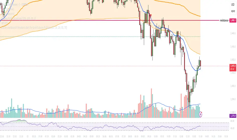
Bullish and Bearish Breakout Alert for Gold Futures PullbackBelow is a Pine Script (version 6) for TradingView that includes both bullish and bearish breakout conditions for my intraday trading strategy on micro gold futures (MGC). The strategy focuses on scalping two-legged pullbacks to the 20 EMA or key levels with breakout confirmation, tailored for the Apex Trader Funding $300K challenge. The script accounts for the Daily Sentiment Index (DSI) at 87 (overbought, favoring pullbacks). It generates alerts for placing stop-limit orders for 175 MGC contracts, ensuring compliance with Apex’s rules ($7,500 trailing threshold, $20,000 profit target, 4:59 PM ET close).
Script Requirements
Version: Pine Script v6 (latest for TradingView, April 2025).
Purpose:
Bullish: Alert when price breaks above a rejection candle’s high after a two-legged pullback to the 20 EMA in a bullish trend (price above 20 EMA, VWAP, higher highs/lows).
Bearish: Alert when price breaks below a rejection candle’s low after a two-legged pullback to the 20 EMA in a bearish trend (price below 20 EMA, VWAP, lower highs/lows).
Context: 5-minute MGC chart, U.S. session (8:30 AM–12:00 PM ET), avoiding overbought breakouts above $3,450 (DSI 87).
Output: Alerts for stop-limit orders (e.g., “Buy: Stop=$3,377, Limit=$3,377.10” or “Sell: Stop=$3,447, Limit=$3,446.90”), quantity 175 MGC.
Apex Compliance: 175-contract limit, stop-losses, one-directional news trading, close by 4:59 PM ET.
How to Use the Script in TradingView
1. Add Script:
Open TradingView (tradingview.com).
Go to “Pine Editor” (bottom panel).
Copy the script from the content.
Click “Add to Chart” to apply to your MGC 5-minute chart .
2. Configure Chart:
Symbol: MGC (Micro Gold Futures, CME, via Tradovate/Apex data feed).
Timeframe: 5-minute (entries), 15-minute (trend confirmation, manually check).
Indicators: Script plots 20 EMA and VWAP; add RSI (14) and volume manually if needed .
3. Set Alerts:
Click the “Alert” icon (bell).
Add two alerts:
Bullish Breakout: Condition = “Bullish Breakout Alert for Gold Futures Pullback,” trigger = “Once Per Bar Close.”
Bearish Breakout: Condition = “Bearish Breakout Alert for Gold Futures Pullback,” trigger = “Once Per Bar Close.”
Customize messages (default provided) and set notifications (e.g., TradingView app, SMS).
Example: Bullish alert at $3,377 prompts “Stop=$3,377, Limit=$3,377.10, Quantity=175 MGC” .
4. Execute Orders:
Bullish:
Alert triggers (e.g., stop $3,377, limit $3,377.10).
In TradingView’s “Order Panel,” select “Stop-Limit,” set:
Stop Price: $3,377.
Limit Price: $3,377.10.
Quantity: 175 MGC.
Direction: Buy.
Confirm via Tradovate.
Add bracket order (OCO):
Stop-loss: Sell 175 at $3,376.20 (8 ticks, $1,400 risk).
Take-profit: Sell 87 at $3,378 (1:1), 88 at $3,379 (2:1) .
Bearish:
Alert triggers (e.g., stop $3,447, limit $3,446.90).
Select “Stop-Limit,” set:
Stop Price: $3,447.
Limit Price: $3,446.90.
Quantity: 175 MGC.
Direction: Sell.
Confirm via Tradovate.
Add bracket order:
Stop-loss: Buy 175 at $3,447.80 (8 ticks, $1,400 risk).
Take-profit: Buy 87 at $3,446 (1:1), 88 at $3,445 (2:1) .
5. Monitor:
Green triangles (bullish) or red triangles (bearish) confirm signals.
Avoid bullish entries above $3,450 (DSI 87, overbought) or bearish entries below $3,296 (support) .
Close trades by 4:59 PM ET (set 4:50 PM alert) .
Multi-Factor Reversal AnalyzerMulti-Factor Reversal Analyzer – Quantitative Reversal Signal System
OVERVIEW
Multi-Factor Reversal Analyzer is a comprehensive technical analysis toolkit designed to detect market tops and bottoms with high precision. It combines trend momentum analysis, price action behavior, wave oscillation structure, and volatility breakout potential into one unified indicator.
This indicator is not a random mix of tools — each module is carefully selected for a specific purpose. When combined, they form a multi-dimensional view of the market, merging trend analysis, momentum divergence, and volatility compression to produce high-confidence signals.
Why Combine These Modules?
Module Combination Ideas & How to Use Them
Factor A: Trend Detector + Gold Zone
Concept:
• The Trend Detector (light yellow histogram) evaluates market strength:
• Histogram trending downward or staying below 50 → bearish conditions;
• Trending upward or staying above 50 → bullish conditions.
• The Gold Zone identifies areas of volatility compression — typically a prelude to explosive market moves.
Practical Application:
• When the Gold Zone appears and the Trend Detector is bearish → likely downside move;
• When the Gold Zone appears and the Trend Detector is bullish → likely upside breakout.
• Note: The Gold Zone does not mean the bottom is in. It is not a buy signal on its own — always combine it with other modules for directional bias.
Factor B: PAI + Wave Trend
Concept:
• PAI (Price Action Index) is a custom oscillator that combines price momentum with volatility dispersion, displaying strength zones:
• Green area → bullish dominance;
• Red area → bearish pressure.
• Wave Trend offers smoothed crossover signals via the main and signal lines.
Practical Application:
• When PAI is in the green zone and Wave Trend makes a bullish crossover → potential reversal to the upside;
• When PAI is in the red zone and Wave Trend shows a bearish crossover → potential start of a downtrend.
Factor C: Trend Detector + PAI
Concept:
• Combines directional trend strength with price action strength to confirm setups via confluence.
Practical Application:
• Trend Detector histogram bottoms out + PAI enters the green zone → high chance of upward reversal;
• Histogram tops out + PAI in the red zone → increased likelihood of downside continuation.
Multi-Factor Confluence (Advanced Use)
• When Trend Detector, PAI, and Wave Trend all align in the same direction (bullish or bearish), the directional signal becomes significantly more reliable.
• This setup is especially useful for trend-following or swing trade entries.
KEY FEATURES
1. Multi-Layer Reversal Logic
• Combines trend scoring, oscillator divergence, and volatility squeezes for triangulated reversal detection.
• Helps traders distinguish between trend pullbacks and true reversals.
2. Advanced Divergence Detection
• Detects both regular and hidden divergences using pivot-based confirmation logic.
• Customizable lookback ranges and pivot sensitivity provide flexible tuning for different market styles.
3. Gold Zone Volatility Compression
• Highlights pre-breakout zones using custom oscillation models (RSI, harmonic, Karobein, etc.).
• Improves anticipation of breakout opportunities following low-volatility compressions.
4. Trend Direction Context
• PAI and Trend Score components provide top-down insight into prevailing bias.
• Built-in “Straddle Area” highlights consolidation zones; breakouts from this area often signal new trend phases.
5. Flexible Visualization
• Color-coded trend bars, reversal markers, normalized oscillator plots, and trend strength labels.
• Designed for both visual discretionary traders and data-driven system developers.
USAGE GUIDELINES
1. Applicable Markets
• Suitable for stocks, crypto, futures, and forex
• Supports reversal, mean-reversion, and breakout trading styles
2. Recommended Timeframes
• Short-term traders: 5m / 15m / 1H — use Wave Trend divergence + Gold Zone
• Swing traders: 4H / Daily — rely on Price Action Index and Trend Detector
• Macro trend context: use PAI HTF mode for higher timeframe overlays
3. Reversal Strategy Flow
• Watch for divergence (WT/PAI) + Gold Zone compression
• Confirm with Trend Score weakening or flipping
• Use Straddle Area breakout for final trigger
• Optional: enable bar coloring or labels for visual reinforcement
• The indicator performs optimally when used in conjunction with a harmonic pattern recognition tool
4. Additional Note on the Gold Zone
The “Gold Zone” does not directly indicate a market bottom. Since it is displayed at the bottom of the chart, it may be misunderstood as a bullish signal. In reality, the Gold Zone represents a compression of price momentum and volatility, suggesting that a significant directional move is about to occur. The direction of that move—upward or downward—should be determined by analyzing the histogram:
• If histogram momentum is weakening, the Gold Zone may precede a downward move.
• If histogram momentum is strengthening, it may signal an upcoming rebound or rally.
Treat the Gold Zone as a warning of impending volatility, and always combine it with trend indicators for accurate directional judgment.
RISK DISCLAIMER
• This indicator calculates trend direction based on historical data and cannot guarantee future market performance. When using this indicator for trading, always combine it with other technical analysis tools, fundamental analysis, and personal trading experience for comprehensive decision-making.
• Market conditions are uncertain, and trend signals may result in false positives or lag. Traders should avoid over-reliance on indicator signals and implement stop-loss strategies and risk management techniques to reduce potential losses.
• Leverage trading carries high risks and may result in rapid capital loss. If using this indicator in leveraged markets (such as futures, forex, or cryptocurrency derivatives), exercise caution, manage risks properly, and set reasonable stop-loss/take-profit levels to protect funds.
• All trading decisions are the sole responsibility of the trader. The developer is not liable for any trading losses. This indicator is for technical analysis reference only and does not constitute investment advice.
• Before live trading, it is recommended to use a demo account for testing to fully understand how to use the indicator and apply proper risk management strategies.
CHANGELOG
v1.0: Initial release featuring integrated Price Action Index, Trend Strength Scoring, Wave Trend Oscillator, Gold Zone Compression Detection, and dual-type divergence recognition. Supports higher timeframe (HTF) synchronization, visual signal markers, and diversified parameter configurations.

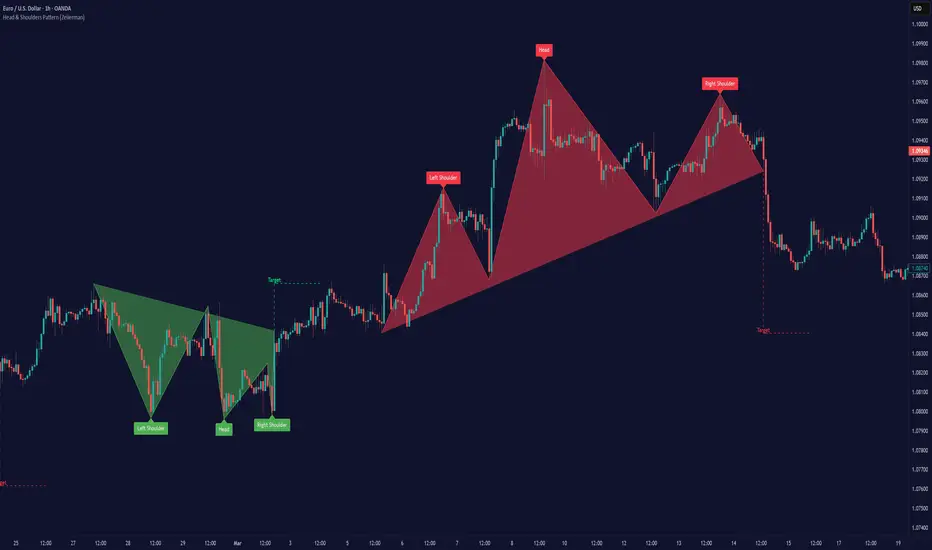
Head & Shoulders Pattern (Zeiierman)█ Overview
The Head & Shoulders Pattern (Zeiierman) is an advanced pattern recognition tool that automatically detects and visualizes one of the most powerful reversal patterns in technical analysis — the classic Head & Shoulders and Inverse Head & Shoulders formations .
This indicator brings structure clarity directly onto the price chart, allowing traders to instantly spot potential major reversal zones without manually drawing or searching for patterns.
It doesn't just draw lines — it intelligently scans price action for symmetry, pivot behavior, and neckline structures — then projects realistic price targets based on the pattern's height.
⚪ In simple terms:
▸ Standard Head & Shoulders → Bearish Reversal Pattern
▸ Inverse Head & Shoulders → Bullish Reversal Pattern
▸ Target Projection → Estimated Move from Neckline Break
▸ Labels → Clear annotation of Left Shoulder, Head, and Right Shoulder
█ How It Works
The indicator combines multiple technical detection layers into a clean visual model:
⚪ Dynamic Pivot Engine
Automatically detects pivot highs and lows based on user-defined Period.
Longer Period = Broader, higher-confidence patterns
Shorter Period = Smaller, more frequent patterns
⚪ Pattern Detection Logic
Scans pivot structures in real-time to identify valid:
Bearish Head & Shoulders (H&S)
Bullish Inverse Head & Shoulders (iH&S)
Conditions include:
▸ Symmetry validation
▸ Head above (or below) Shoulders
▸ Neckline structure
▸ Minimum price conditions met
█ How to Use
⚪ Reversal Trading
Look for Head & Shoulders at the top of an uptrend
Look for Inverse Head & Shoulders at the bottom of a downtrend
⚪ What makes our tool truly unique is that it goes beyond the traditional textbook definition.
Our custom Head & Shoulders algorithm is built with flexibility and adaptability in mind. It dynamically responds to real-time price action, allowing it to detect valid patterns not only at major trend reversals — but also within trending environments.
That means you can spot Head & Shoulders formations at:
Consolidation zones
Trend continuation areas
Corrective phases within established trends
It doesn’t have to be the absolute top or bottom of a move — and that’s the real power of this tool. It adapts. It evolves. It finds structure where most indicators stay blind.
█ Common Real-World Stop Loss Strategies with Head & Shoulders Patterns
Not all Head & Shoulders patterns are created equal — and neither are the stop loss strategies used to trade them.
Depending on your trading style, risk tolerance, and market context — here are the 3 most common ways traders manage stop placement when trading Head & Shoulders (H&S) or Inverse Head & Shoulders (iH&S) patterns:
⚪ Conservative Stop Placement
Maximum Safety — Minimum Chance of Being Stopped Prematurely
Stop Placement:
Above the Head (Bearish H&S)
Below the Head (Bullish iH&S)
Pros: Safest approach. Provides maximum protection against false breakouts and noise.
Cons: Often results in very large stop losses, especially on bigger patterns or higher timeframes. Risk-to-Reward (RR) can be poor unless the target is far.
⚪ Aggressive Stop Placement
Tighter Risk — Faster Invalidations
Stop Placement:
Above the Right Shoulder (Bearish H&S)
Below the Right Shoulder (Bullish iH&S)
Pros: Smaller stop losses. Improved RR. Ideal for traders who want tighter control over risk.
Cons: Higher chance of getting stopped on retests or minor volatility around the neckline zone.
⚪ Neckline Reclaim Invalidation
Dynamic & Price-Action Based Exit
Stop Placement:
Exit the trade if price closes back above (bearish) or below (bullish) the neckline after breaking it.
Pros: Dynamic approach based on market behavior rather than static levels. Allows more flexibility.
Cons: Requires active trade management. Not suitable for fully automated or set-and-forget trading styles.
█ Why It's Useful
This is not a basic pattern drawing tool — it's a complete detection system built for traders who want to:
Automatically detect powerful reversal patterns
Avoid the subjectivity of manually drawing H&S structures
Trade with clear target projections
Identify high-probability reversal zones
Visually map structure shifts in real-time
█ Settings
Pivot Detection
Period → Number of bars used to scan for pivots (Higher = Bigger patterns)
Pattern Detection
Enable Bullish Head & Shoulders
Enable Bearish Head & Shoulders
Visualization
Customize Colors (Lines, Fills, Labels)
Enable/Disable Labels
Pattern Style: Closed / Open
Custom Label Colors
Target Projection
Enable/Disable Target Projection
Customize Target Colors
-----------------
Disclaimer
The content provided in my scripts, indicators, ideas, algorithms, and systems is for educational and informational purposes only. It does not constitute financial advice, investment recommendations, or a solicitation to buy or sell any financial instruments. I will not accept liability for any loss or damage, including without limitation any loss of profit, which may arise directly or indirectly from the use of or reliance on such information.
All investments involve risk, and the past performance of a security, industry, sector, market, financial product, trading strategy, backtest, or individual's trading does not guarantee future results or returns. Investors are fully responsible for any investment decisions they make. Such decisions should be based solely on an evaluation of their financial circumstances, investment objectives, risk tolerance, and liquidity needs.
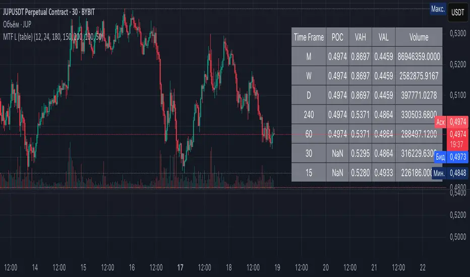
Multi-Timeframe Liquidity Zones V6 (Table)Multi-Timeframe Liquidity Zones V6 (Table) Indicator: Functionality and Uses
Overview: The Multi-Timeframe Liquidity Zones V6 (Table) indicator is a technical analysis tool that highlights key volume-based support and resistance levels across multiple timeframes. It leverages volume profile concepts – specifically the Point of Control (POC) and Value Area High/Low (VAH/VAL) – to identify “liquidity zones” where trading activity was heaviest . Unlike a standard single-timeframe volume profile, this indicator compiles data from several timeframes (e.g. monthly, weekly, daily, intraday) and displays the results in a convenient table format on the chart. The goal is to give traders a consolidated view of important price levels (derived from volume concentrations) across different horizons, helping them plan trades with a broader market perspective.
Purpose and Functionality of the Indicator
Multi-Timeframe Analysis: The primary objective of this indicator is to simplify multi-timeframe analysis of volume distribution. Rather than manually checking volume profiles on separate charts for each timeframe, the tool automatically calculates the key levels for each selected timeframe and presents them together. This includes higher-level perspectives (like monthly or weekly volume hotspots) alongside shorter-term levels (daily or hourly), ensuring that traders don’t miss significant zones from any timeframe . By offering a broader perspective on support and resistance levels, multi-timeframe tools help improve risk management and signal confirmation , and this indicator is designed to provide that volume-based perspective at a glance.
Table Format Display: Multi-Timeframe Liquidity Zones V6 (Table) specifically presents the information as a table (as opposed to plotting lines on the chart). Each row in the table typically corresponds to a timeframe (for example, Monthly, Weekly, Daily, 4H, 1H, 30M, 15M), and the columns list the calculated POC, VAH, VAL, and possibly the average volume for that timeframe’s look-back period. By structuring the data in a table, traders can quickly read off the exact price levels of these liquidity zones without having to visually trace lines. This format makes it easy to compare levels across timeframes or note where multiple timeframes’ levels cluster near the same price – a sign of especially strong support/resistance. The indicator uses a user-defined number of bars or length of history for each timeframe to calculate these values (so you can adjust how far back it looks to define the volume profile for each period).
Objective: In summary, the functionality is geared toward identifying high-liquidity price zones across multiple time scales and presenting them clearly. These high-liquidity zones often coincide with areas where price reacts (stalls, reverses, or accelerates) because a lot of trading activity (hence, orders and volume) took place there in the past. The indicator’s objective is to alert the trader to those areas in advance. It effectively answers questions like: “Where are the major volume concentration levels on the 1-hour, daily, and weekly charts right now?” and “Are there overlapping volume-based support/resistance levels from different timeframes around the current price?” By compiling this information, the indicator helps traders incorporate context from multiple timeframes in their decision-making, without needing to flip through numerous charts.
Identifying Liquidity Zones with POC, VAH, and VAL
Liquidity Zones Defined: In market terms, a “liquidity zone” is an area of the chart where a significant amount of trading occurred, meaning high liquidity (many buyers and sellers exchanged volume there). These zones often act as support or resistance because past heavy trading indicates consensus or interest around those price levels. This indicator identifies liquidity zones through volume profile analysis on each timeframe’s recent price action. Essentially, it looks at the distribution of trading volume at different prices over the specified period and finds the value area – the range of prices that encompassed the majority of that volume (commonly around 70% of the total volume ). Within that value area, it pinpoints the Point of Control (POC), which is the single price level that had the highest traded volume (the peak of the volume profile) . The upper and lower boundaries of that high-volume range are marked as Value Area High (VAH) and Value Area Low (VAL) respectively . Together, the VAH and VAL define the liquidity zone where the market spent most of its time and volume, and POC highlights the most traded price in that zone.
• Point of Control (POC): The POC is the price level with the greatest volume traded for the given period. It represents the price at which the most liquidity was exchanged – effectively the market’s “center of gravity” for that timeframe’s trading activity . The indicator calculates the POC for each selected timeframe by scanning the volume at each price; the price with maximum volume is flagged as that timeframe’s POC. In the table, the POC might be highlighted or listed as a key level (sometimes traders color-code it or mark it for emphasis). Because so many positions were opened or closed at the POC, it often serves as a strong support/resistance. For example, if price falls to a major POC from above, traders expect buyers may step in there (since it was a popular buy/sell level historically), potentially causing a bounce. Conversely, if price breaks through a POC decisively, it may signal a significant shift in market acceptance.
• Value Area High (VAH) and Low (VAL): The VAH and VAL are the price boundaries of the value area, which is typically defined to contain about 70% of the total traded volume for the period . In other words, between VAH and VAL is where the “bulk” of trading occurred, and outside this range is where relatively less volume traded. The indicator derives VAH/VAL by accumulating volume from the highest-volume price (POC) outward until ~70% of volume is covered (this is a common method for volume profile value area). VAH is the top of this high-volume region and VAL is the bottom. These levels are important because they often act like support/resistance boundaries: when price is inside the value area, it’s in a high-liquidity zone and tends to oscillate between VAH and VAL; when price moves above VAH or below VAL, it’s leaving the high-volume zone, which can indicate a potential trend or imbalance (price entering a lower-liquidity area where it might move faster until finding the next liquidity zone). Traders watch VAH/VAL for signs of rejection or acceptance: for instance, a price rally that falters at VAH suggests that level is acting as resistance (sellers defending that high-volume area), whereas if price pushes above VAH, it may continue until the next timeframe’s zone or until it finds new interest. The Multi-Timeframe Liquidity Zones V6 indicator gives the VAH and VAL for each timeframe, essentially mapping out the upper and lower bounds of key liquidity zones at those scales.
How the Indicator Identifies These: Under the hood, the indicator likely uses historical price and volume data for each timeframe’s lookback window. For each timeframe (say the last 20 weekly bars for a weekly profile, last 100 daily bars for a daily profile, etc.), it constructs a volume profile (a histogram of volume at each price). From that distribution, it finds the POC (highest volume bin) and calculates VAH/VAL around it. The output is a set of numbers (price levels) that mark where those zones lie. In practice, if using the Lines version of this indicator, those levels are drawn as horizontal lines on the chart and labeled by timeframe (e.g., a line at 1.2345 labeled “D POC” for Daily POC) . In the Table version, those values are instead listed in text form. Either way, the identification process is the same – it’s finding the high-volume price regions on each timeframe and calling them out. By doing this for multiple timeframes concurrently, the indicator reveals how these liquidity zones from different periods relate to each other. For example, you might discover that a daily-chart value area overlaps with a weekly-chart POC, creating a particularly strong zone of interest. This kind of insight is hard to get from a single timeframe analysis alone.
Volume Profile Data Across Multiple Timeframes
Multiple Timeframes in One View: One of the biggest advantages of this indicator is the ability to see volume profile information from various timeframes side by side. Traders often perform multiple timeframe analysis to get a fuller picture — for instance, checking monthly or weekly levels for long-term context while planning a trade on a 4-hour chart. This indicator automates that process for volume-based levels. The table will typically list each chosen timeframe (which could be preset or user-selected). For each timeframe, you get the POC, VAH, VAL, and possibly an average volume metric. The “average volume” likely refers to the average volume per bar or the average volume traded over the profile’s duration for that timeframe, which gives a sense of how significant that period’s activity is. For example, a weekly profile might show an average volume of say 500k per week, versus a daily profile average of 80k per day – indicating the scale of trading on weekly vs daily. High average volume on a timeframe means its liquidity zones were formed with a lot of participation, possibly making them more reliable support/resistance. By comparing these, traders can gauge which timeframes had unusually high or low activity recently. The table format makes such comparisons straightforward.
Identification of Confluence: Because all the data is presented together, traders can quickly spot confluence or overlaps between timeframes. If two different timeframes show liquidity zones at similar price levels, that price becomes extremely noteworthy. For instance, suppose the indicator shows: a 1-hour POC at 1.1300, a 4-hour VAL at 1.1280, and a daily VAL at 1.1290. These are all in a tight range – effectively indicating a multi-timeframe liquidity zone around 1.1280–1.1300. A trader seeing this cluster in the table will recognize that as a strong support area, since multiple profiles from intraday to daily all suggest heavy trading interest there. Similarly, overlaps of VAH (resistance zone) from different timeframes could signal a strong ceiling. The multi-timeframe view prevents a trader from, say, going long into a major weekly POC above, or shorting when there’s a huge monthly value-area low just below – situations where awareness of higher timeframe volume structure can make the difference between a good and bad trade.
User Customization: The indicator is flexible in that you can typically adjust which timeframes to include and how many bars to use for each timeframe’s calculation. For example, one might configure it to calculate monthly levels using the past 12 monthly bars (1 year of data), weekly levels using the past 20 weeks, daily using 100 days, etc., depending on preference. By tuning the “bars count” or period length , the trader can focus on recent liquidity zones or incorporate more history if desired. Shorter lookback might catch more recent shifts in volume distribution (important if the market structure changed recently), while longer lookback gives more established levels. This customization ensures the indicator’s output can be tailored to different trading styles (short-term vs swing vs long-term investing). Regardless of settings, the multi-timeframe table allows simultaneous visibility of the chosen timeframes’ volume landscape. This comprehensive view is the core strength: it consolidates data that normally requires flipping through multiple charts.
Using the Liquidity Zones Data for Trading Decisions
Traders can use the information from the MTF Liquidity Zones V6 (Table) indicator in several practical ways to enhance their decision-making:
• Identify Support and Resistance: Each liquidity zone acts as a potential support or resistance area. For example, if the table shows a daily VAH at a certain level above the current price, that level might serve as resistance if the price rallies up to it (since it marks the top of a high-volume region where sellers might step in). Conversely, a weekly VAL below current price could act as support on a dip. By noting these levels in the table, a trader planning an entry or exit can anticipate where the price might stall or reverse. Essentially, you get a map of high-interest price levels from different timeframes, which you can mark on your trading chart for guidance.
• Plan Entries and Exits Around Key Levels: Many traders incorporate volume profile levels into their strategies, for instance: buying near VAL (betting that the value area will hold and price will revert upward), or selling/shorting near VAH (expecting the top of value to hold as resistance), or trading breakouts when price moves outside the value area. With the multi-timeframe table, one can refine these tactics by also considering higher timeframe levels. Suppose you see that on the 1-hour chart the price is just above its 1H POC, but the table indicates that just slightly above, there’s also the daily POC. You might delay a long entry until price clears that daily POC, because that could be a stronger intraday barrier. Or if you intend to take profit on a long trade, you might choose a target just below a weekly VAH since price may struggle to climb past that on the first attempt. The indicator thus acts as a guide for precision in entry/exit decisions, aligning them with where liquidity is high.
• Gauge Trend Strength and Directional Bias: By observing where current price is relative to these volume zones, traders can infer certain market conditions. For instance, if price is trading above the VAH of multiple timeframes’ value areas, it suggests the market is in a more bullish or overextended territory (price accepted above prior value), whereas if price is below multiple VALs, it’s in bearish or undervalued territory relative to recent history. If the price stays around a POC, it indicates consolidation or equilibrium (market comfortable at that price). Traders can use this context for bias – e.g., if price is above the weekly VAH, you might lean bullish but watch for potential pullbacks to that VAH level (now a support). If price is below the monthly VAL, you might avoid longs until it re-enters that value area. In essence, the liquidity zones provide context of value vs. price: is price trading within the high-volume areas (implying range-bound behavior) or outside them (implying a breakout or trending move)? This can prevent chasing trades at poor locations.
• Combine with Other Indicators/Analysis: It’s generally advised to not use any single indicator in isolation, and this holds true here. The liquidity zones from this indicator are best used alongside price action or other technical signals for confirmation . For example, if a bullish candlestick reversal pattern forms right at a confluence of a 4H VAL and Daily POC, that’s a stronger buy signal than the pattern alone. Or if an oscillator shows overbought exactly as price hits a weekly VAH, it adds conviction to a possible short. The indicator’s table basically gives you a shortlist of critical price levels; you can then watch how price behaves at those levels (via candlesticks, order flow, etc.) to make the final trade decision. Traders might set alerts for when price approaches one of the listed levels, or they might drop down to a lower timeframe to fine-tune an entry once a key zone is reached. By integrating this volume-based insight with trend analysis, chart patterns, or momentum indicators, one can make more informed and high-probability decisions rather than trading in the dark.
• Risk Management and Stop Placement: High-liquidity zones can also inform stop-loss placement. Ideally, you want your stop on the other side of a strong support/resistance. If you go long near a VAL, you might place your stop just below the VAL (since a move beyond that suggests the high-volume zone didn’t hold). If you short near a VAH, a stop just above the VAH or POC could be logical. Moreover, if multiple timeframes show overlapping zones, a stop beyond all of them could be even safer (albeit at the cost of a wider stop). The indicator helps identify those spots. It also warns you of where not to put a stop – for example, placing a stop-loss right at a POC might be unwise because price could gravitate to that POC repeatedly (due to its magnetic effect as a high-volume price). Instead, a trader might choose a stop beyond the far side of the value area. By using the table’s information, you can align your risk management with areas of high liquidity, reducing the chance of being whipsawed by normal volatility around heavily traded levels .
Benefits of the Multi-Timeframe Liquidity Zones Indicator
Using the Multi-Timeframe Liquidity Zones V6 (Table) indicator offers several key benefits for traders, ultimately aiming to streamline analysis and improve decision quality:
• Consolidated Key Levels: It provides a clear, consolidated view of crucial volume-driven levels from multiple timeframes all at once . This saves time and ensures you always account for major support/resistance zones that come from higher or lower timeframe volume clusters. You won’t accidentally overlook a significant weekly level while focused on a 15-minute chart, for example.
• Enhanced Multi-Timeframe Insight: By aligning information from long-term and short-term periods, the indicator helps traders see the “bigger picture” while still operating on their preferred timeframe. This multi-scale awareness can improve trade timing and confidence. You’re effectively doing multi-timeframe analysis with volume profiles in an efficient manner, which can confirm or caution your trade ideas (e.g., a trend looks strong on the 1H, but the table shows a huge monthly VAH just overhead – a reason to be cautious or take profit early).
• Improved Decision Making and Precision: Knowing where liquidity zones lie allows for more precise entries, exits, and stop placements. Traders can make informed decisions such as waiting for a pullback to a value area before entering, or taking profits before price hits a major POC from a higher timeframe. These decisions are grounded in objectively important price levels, potentially leading to higher probability trades and better risk-reward setups. It essentially enhances your strategy by adding a layer of volume context – you’re trading with an awareness of where the market’s interest is heaviest.
• Volume-Based Confirmation: Price alone can sometimes be deceptive, but volume tells the true story of participation. The liquidity zones indicator provides volume-based confirmation of support/resistance. If a price level is identified by this tool, it’s because significant volume happened there – adding weight to that level’s importance. This can help filter out false support/resistance levels that aren’t backed by volume. In other words, it highlights high-quality levels that many traders (and possibly institutions) have shown interest in.
• Adaptable to Different Trading Styles: Whether one is a scalper looking at intraday (15M, 5M charts) or a swing trader focusing on daily/weekly, the indicator can be configured to those needs. You choose which timeframes and how much data to consider. This means the concept of liquidity zones can be applied universally – from spotting intraday pivot levels with volume, to seeing long-term value zones on an investment. The consistent methodology of POC/VAH/VAL across scales provides a common framework to analyze any market and timeframe.
• Informed Risk Management: As discussed, the knowledge of multi-timeframe volume zones aids in risk management. By placing stops beyond major liquidity areas or avoiding trades that run into strong volume walls, traders can reduce the likelihood of whipsaw losses. It’s an extra layer of defense to ensure your trade plan accounts for where the market has historically found lots of interest (hence likely friction). This level of informed planning can be the difference between a well-managed trade and an avoidable loss.
In conclusion, the Multi-Timeframe Liquidity Zones V6 (Table) indicator serves as a powerful analytical aid, giving traders a structured view of where price is likely to encounter support or resistance based on volume concentrations across timeframes. Its functionality centers on identifying those liquidity zones (via POC, VAH, VAL) and presenting them in an easy-to-read format, while its ultimate purpose is to help traders make more informed decisions. By integrating this tool into their workflow, traders can more confidently navigate price action, knowing the objective volume-based landmarks that lie ahead. Remember that while these volume levels often coincide with strong S/R zones, it’s best to use them in conjunction with other technical or fundamental analysis for confirmation . When used appropriately, the indicator can streamline multi-timeframe analysis and enhance your overall trading strategy , giving you an edge in identifying where the market’s liquidity (and opportunity) resides.
Supertrend ProSupertrend Pro - Multi-Trend Analysis and Trading Signal Filtering
OVERVIEW
This indicator calculates trend direction based on the Supertrend indicator and integrates dual-trend analysis, upper and lower trend bands, trading signal alerts, moving average filtering, and the EMA 200 bull-bear division line to provide traders with more precise trend identification and trading signals.
It is suitable for trend trading, short-term trading, and swing trading, effectively filtering market noise and improving trade accuracy.
IMPLEMENTATION PRINCIPLES
1. Primary Trend: Uses the Supertrend indicator to calculate major trend direction, suitable for long-term trend assessment.
2. Secondary Trend: Detects short-term trend changes, capturing finer market movements.
3. Upper and Lower Trend Bands: Utilizes ATR (Average True Range) to calculate dynamic trend channels, assisting in trend strength assessment.
4. Trading Signal Alerts: Provides buy/sell signals when trends reverse, with optional moving average filtering to reduce false signals.
5. Moving Average Filtering: Supports multiple MA types, such as EMA, SMA, HMA, McGinley, helping to filter market noise.
6. EMA 200 Bull-Bear Division Line: Combines ATR-based trend buffer zones to distinguish between long-term bull and bear markets, enhancing trend accuracy.
KEY FEATURES
1. Dual-Trend Analysis
• Primary trend is suitable for long-term trend tracking, reducing interference from short-term fluctuations.
• Secondary trend is ideal for short-term trading opportunities, allowing faster identification of market turning points.
• By combining both, traders can follow the major trend direction while using the secondary trend for optimized entry points, improving trade success rates.
2. Upper and Lower Trend Bands
• ATR-based dynamic bands adjust to market volatility, avoiding the limitations of fixed support and resistance levels.
• Trend confirmation: When the price reaches the upper or lower band, traders can determine whether the market is overheated or oversold, aiding trading decisions.
• Combining primary and secondary trend bands provides clearer trend validation, reducing false signals.
3. Trading Signal Alerts
• Automatic buy/sell signal alerts when the trend reverses, eliminating the need for manual trend assessment.
• Moving average filtering improves signal reliability, reducing false signals.
• Supports various signal markers (circles/arrows/labels) to help traders clearly visualize entry points.
4. Moving Average Filtering
• Supports multiple moving average types (SMA, EMA, HMA, WMA, McGinley, etc.), adapting to different trading styles.
• Prevents counter-trend trading:
· Long entries only when the price is above the MA filter.
· Short entries only when the price is below the MA filter.
• Customizable MA periods to suit different market conditions and prevent excessive signal noise.
5. Trading Reference Lines
• Short-term trend: HMA 25 serves as an entry reference line. Waiting for MA color changes before placing trades can improve stability.
• Long-term trend: EMA 200 as the bull-bear division line helps traders distinguish between long-term bullish and bearish trends, avoiding counter-trend trades.
• Dynamic buffer adjustment: Uses ATR-based volatility buffers to reduce false signals and enhance trend detection accuracy.
• Color-coded trend identification:
· Aqua (Bull Market): Price is above the buffer zone.
· Fuchsia (Bear Market): Price is below the buffer zone.
· White: Price is within the buffer zone, indicating an unclear market direction.
USAGE GUIDELINES
1. Applicable Markets
• Suitable for stocks, futures, cryptocurrencies, and forex
• Supports short-term trading, trend trading, and swing trading
2. Recommended Timeframes
• Short-term traders can use 5m, 15m, and 1H timeframes, leveraging secondary trend signals for quick market entries.
• Trend traders can use 4H and daily timeframes, relying on primary trend signals to assess major trends.
• Long-term investors can use the EMA 200 bull-bear division line to determine macro trend direction and avoid counter-trend trades.
3. Trading Strategy
• Long Entry:
The primary trend is bullish (Green).
The secondary trend triggers a buy signal (Long).
• Short Entry:
· The primary trend is bearish (Red).
· The secondary trend triggers a sell signal (Short).
• Enable Moving Average Filtering:
· Only enter long trades when the price is above the MA filter.
· Only enter short trades when the price is below the MA filter.
• Use EMA 200 for Market Direction:
· If the price is above EMA 200 + buffer, the market is in a bullish trend → favor long trades.
· If the price is below EMA 200 - buffer, the market is in a bearish trend → favor short trades.
• Market Volatility Considerations:
· Short timeframes (1m, 5m) may produce more noise, reducing signal reliability.
· Higher timeframes (1H, 4H, Daily) provide more stable trend signals but may miss some short-term trade opportunities.
RISK DISCLAIMER
• This indicator calculates trend direction based on historical data and cannot guarantee future market performance. When using this indicator for trading, always combine it with other technical analysis tools, fundamental analysis, and personal trading experience for comprehensive decision-making.
• Market conditions are uncertain, and trend signals may result in false positives or lag. Traders should avoid over-reliance on indicator signals and implement stop-loss strategies and risk management techniques to reduce potential losses.
• Leverage trading carries high risks and may result in rapid capital loss. If using this indicator in leveraged markets (such as futures, forex, or cryptocurrency derivatives), exercise caution, manage risks properly, and set reasonable stop-loss/take-profit levels to protect funds.
• All trading decisions are the sole responsibility of the trader. The developer is not liable for any trading losses. This indicator is for technical analysis reference only and does not constitute investment advice.
• Before live trading, it is recommended to use a demo account for testing to fully understand how to use the indicator and apply proper risk management strategies.
CHANGELOG
• v1.0: Initial release with a dual-trend system, dynamic upper and lower trend bands, trading signal alerts, moving average filtering, HMA trading reference line, and EMA 200 bull-bear division.

Wick Size in USD with 10-Bar AverageWick Size in USD with 10-Bar Average
Version: 1.0
Author: QCodeTrader
🔍 Overview
This indicator converts the price wicks of your candlestick chart into USD values based on ticks, providing both raw and smoothed data via a 10-bar simple moving average. It helps traders visualize the monetary impact of price extremes, making it easier to assess volatility, potential risk, and plan appropriate stop loss levels.
⚙️ Key Features
Tick-Based Calculation:
Converts wick sizes into ticks (using a fixed tick size of 0.01, typical for stocks) and then into USD using a customizable tick value.
10-Bar Moving Average:
Smooths out the wick values over the last 10 bars, giving you a clearer view of average wick behavior.
Bullish/Bearish Visual Cues:
The chart background automatically highlights bullish candles in green and bearish candles in red for quick visual assessment.
Stop Loss Optimization:
The indicator highlights long wick sizes, which can help you set more accurate stop loss levels. Even when the price moves in your favor, long wicks may indicate potential reversals—allowing you to account for this risk when planning your stop losses.
User-Friendly Customization:
Easily adjust the USD value per tick through the settings to tailor the indicator to your specific instrument.
📊 How It Works
Wick Calculation:
The indicator calculates the upper and lower wicks by measuring the distance between the candle’s high/low and its body (open/close).
Conversion to Ticks & USD:
These wick sizes are first converted from price points to ticks (dividing by a fixed tick size of 0.01) and then multiplied by the user-defined tick value to convert the measurement into USD.
Smoothing Data:
A 10-bar simple moving average is computed for both the upper and lower wick values, providing smoothed data that helps identify trends and deviations.
Visual Representation:
Columns display the raw wick sizes in USD.
Lines indicate the 10-bar moving averages.
Background Color shifts between green (bullish) and red (bearish) based on candle type.
⚡ How to Use
Add the Indicator:
Apply it to your chart to begin visualizing wick sizes in monetary terms.
Customize Settings:
Adjust the Tick Value in USD in the settings to match your instrument’s tick value.
(Note: The tick size is fixed at 0.01, which is standard for many stocks.)
Optimize Your Stop Loss:
Analyze the raw and averaged wick values to understand volatility. Long wicks—even when the price moves in your favor—may indicate potential reversals. This insight can help you set more accurate stop loss levels to protect your gains.
Analyze:
Use the indicator’s data to gauge market volatility and assess the significance of price movements, aiding in more informed trading decisions.
This indicator is perfect for traders looking to understand the impact of extreme price movements in monetary terms, optimize stop loss levels, and effectively manage risk across stocks and other instruments with similar tick structures.
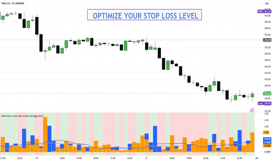
Pivot High/Low [s3]This is a technical analysis tool that identifies significant price pivot points (highs and lows) in the market. It looks for both major and minor pivot points, which can help traders identify potential support and resistance levels, trend reversals, and breakout opportunities.
How Pivot Points Are Calculated:
The indicator uses a straightforward "higher than everything around it" or "lower than everything around it" approach:
For Pivot Highs:
- The indicator looks at a specific bar and compares it to bars before and after it
- For a major pivot high: It checks 50 bars to the left and 20 bars to the right
- If the bar's high price is higher than ALL bars within this range, it's marked as a pivot high
- Think of it like a mountain peak - it needs to be the highest point compared to everything around it
For Pivot Lows:
- Same concept but reversed - looking for valleys instead of peaks
- Checks the same ranges (50 left, 20 right)
- The bar's low price must be lower than ALL surrounding bars
- Like finding the bottom of a valley - it needs to be the lowest point in the area
Key Features:
1. Two types of pivot points:
- Major pivots (using longer lookback periods of 50 bars left, 20 bars right)
- Minor pivots (using half the lookback periods - 25 left, 10 right)
2. Visual elements:
- Triangle markers above/below bars for pivot points
- Dotted lines extending from pivot points
- Color coding: Green for lows (support), Red for highs (resistance)
- Major pivots are more prominent than minor pivots
3. Customizable alerts for:
- Formation of new pivot points
- Breakouts above/below pivot levels
Trading Applications:
1. Support and Resistance:
- Major pivot levels act as strong support (lows) and resistance (highs)
- Multiple touches of these levels increase their significance
- Minor pivots can indicate intermediate support/resistance levels
2. Trend Analysis:
- Higher highs and higher lows = Uptrend
- Lower highs and lower lows = Downtrend
- Breaking of major pivot levels can signal trend changes
3. Entry/Exit Signals:
- Long entries: When price bounces off major pivot lows
- Short entries: When price rejects from major pivot highs
- Take profits: At opposite pivot levels
- Stop losses: Just beyond the entry pivot level
4. Breakout Trading:
- Breaking above major pivot highs suggests bullish momentum
- Breaking below major pivot lows suggests bearish momentum
- Use the alert system to catch breakouts early
Settings Customization:
- Adjust lookback periods based on your timeframe
- Toggle visibility of markers and lines
- Customize colors for better visibility
- Enable/disable specific types of alerts
Risk Management Tips:
1. Don't rely solely on pivot points - combine with other indicators
2. Wait for confirmation of bounces/rejections before entering trades
3. Use proper position sizing based on stop loss placement
4. Consider market context and overall trend when trading pivot levels
This indicator is particularly useful for swing traders and position traders who focus on key market turning points and trend changes. It helps identify significant price levels where the market has previously shown reaction, making it valuable for both trend following and counter-trend strategies.

Quantify [Entry Model] | FractalystWhat’s the indicator’s purpose and functionality?
Quantify is a machine learning entry model designed to help traders identify high-probability setups to refine their strategies.
➙ Simply pick your bias, select your entry timeframes, and let Quantify handle the rest for you.
Can the indicator be applied to any market approach/trading strategy?
Absolutely, all trading strategies share one fundamental element: Directional Bias
Once you’ve determined the market bias using your own personal approach, whether it’s through technical analysis or fundamental analysis, select the trend direction in the Quantify user inputs.
The algorithm will then adjust its calculations to provide optimal entry levels aligned with your chosen bias. This involves analyzing historical patterns to identify setups with the highest potential expected values, ensuring your setups are aligned with the selected direction.
Can the indicator be used for different timeframes or trading styles?
Yes, regardless of the timeframe you’d like to take your entries, the indicator adapts to your trading style.
Whether you’re a swing trader, scalper, or even a position trader, the algorithm dynamically evaluates market conditions across your chosen timeframe.
How can this indicator help me to refine my trading strategy?
1. Focus on Positive Expected Value
• The indicator evaluates every setup to ensure it has a positive expected value, helping you focus only on trades that statistically favor long-term profitability.
2. Adapt to Market Conditions
• By analyzing real-time market behavior and historical patterns, the algorithm adjusts its calculations to match current conditions, keeping your strategy relevant and adaptable.
3. Eliminate Emotional Bias
• With clear probabilities, expected values, and data-driven insights, the indicator removes guesswork and helps you avoid emotional decisions that can damage your edge.
4. Optimize Entry Levels
• The indicator identifies optimal entry levels based on your selected bias and timeframes, improving robustness in your trades.
5. Enhance Risk Management
• Using tools like the Kelly Criterion, the indicator suggests optimal position sizes and risk levels, ensuring that your strategy maintains consistency and discipline.
6. Avoid Overtrading
• By highlighting only high-potential setups, the indicator keeps you focused on quality over quantity, helping you refine your strategy and avoid unnecessary losses.
How can I get started to use the indicator for my entries?
1. Set Your Market Bias
• Determine whether the market trend is Bullish or Bearish using your own approach.
• Select the corresponding bias in the indicator’s user inputs to align it with your analysis.
2. Choose Your Entry Timeframes
• Specify the timeframes you want to focus on for trade entries.
• The indicator will dynamically analyze these timeframes to provide optimal setups.
3. Let the Algorithm Analyze
• Quantify evaluates historical data and real-time price action to calculate probabilities and expected values.
• It highlights setups with the highest potential based on your selected bias and timeframes.
4. Refine Your Entries
• Use the insights provided—entry levels, probabilities, and risk calculations—to align your trades with a math-driven edge.
• Avoid overtrading by focusing only on setups with positive expected value.
5. Adapt to Market Conditions
• The indicator continuously adapts to real-time market behavior, ensuring its recommendations stay relevant and precise as conditions change.
How does the indicator calculate the current range?
The indicator calculates the current range by analyzing swing points from the very first bar on your charts to the latest available bar it identifies external liquidity levels, also known as BSLQ (buy-side liquidity levels) and SSLQ (sell-side liquidity levels).
What's the purpose of these levels? What are the underlying calculations?
1. Understanding Swing highs and Swing Lows
Swing High: A Swing High is formed when there is a high with 2 lower highs to the left and right.
Swing Low: A Swing Low is formed when there is a low with 2 higher lows to the left and right.
2. Understanding the purpose and the underlying calculations behind Buyside, Sellside and Pivot levels.
3. Identifying Discount and Premium Zones.
4. Importance of Risk-Reward in Premium and Discount Ranges
How does the script calculate probabilities?
The script calculates the probability of each liquidity level individually. Here's the breakdown:
1. Upon the formation of a new range, the script waits for the price to reach and tap into pivot level level. Status: "■" - Inactive
2. Once pivot level is tapped into, the pivot status becomes activated and it waits for either liquidity side to be hit. Status: "▶" - Active
3. If the buyside liquidity is hit, the script adds to the count of successful buyside liquidity occurrences. Similarly, if the sellside is tapped, it records successful sellside liquidity occurrences.
4. Finally, the number of successful occurrences for each side is divided by the overall count individually to calculate the range probabilities.
Note: The calculations are performed independently for each directional range. A range is considered bearish if the previous breakout was through a sellside liquidity. Conversely, a range is considered bullish if the most recent breakout was through a buyside liquidity.
What does the multi-timeframe functionality offer?
You can incorporate up to 4 higher timeframe probabilities directly into the table.
This feature allows you to analyze the probabilities of buyside and sellside liquidity across multiple timeframes, without the need to manually switch between them.
By viewing these higher timeframe probabilities in one place, traders can spot larger market trends and refine their entries and exits with a better understanding of the overall market context.
What are the multi-timeframe underlying calculations?
The script uses the same calculations (mentioned above) and uses security function to request the data such as price levels, bar time, probabilities and booleans from the user-input timeframe.
How does the Indicator Identifies Positive Expected Values?
Quantify instantly calculates whether a trade setup has the potential to generate positive expected value (EV).
To determine a positive EV setup, the indicator uses the formula:
EV = ( P(Win) × R(Win) ) − ( P(Loss) × R(Loss))
where:
- P(Win) is the probability of a winning trade.
- R(Win) is the reward or return for a winning trade, determined by the current risk-to-reward ratio (RR).
- P(Loss) is the probability of a losing trade.
- R(Loss) is the loss incurred per losing trade, typically assumed to be -1.
By calculating these values based on historical data and the current trading setup, the indicator helps you understand whether your trade has a positive expected value.
How can I know that the setup I'm going to trade with has a positive EV?
If the indicator detects that the adjusted pivot and buy/sell side probabilities have generated positive expected value (EV) in historical data, the risk-to-reward (RR) label within the range box will be colored blue and red .
If the setup does not produce positive EV, the RR label will appear gray.
This indicates that even the risk-to-reward ratio is greater than 1:1, the setup is not likely to yield a positive EV because, according to historical data, the number of losses outweighs the number of wins relative to the RR gain per winning trade.
What is the confidence level in the indicator, and how is it determined?
The confidence level in the indicator reflects the reliability of the probabilities calculated based on historical data. It is determined by the sample size of the probabilities used in the calculations. A larger sample size generally increases the confidence level, indicating that the probabilities are more reliable and consistent with past performance.
How does the confidence level affect the risk-to-reward (RR) label?
The confidence level (★) is visually represented alongside the probability label. A higher confidence level indicates that the probabilities used to determine the RR label are based on a larger and more reliable sample size.
How can traders use the confidence level to make better trading decisions?
Traders can use the confidence level to gauge the reliability of the probabilities and expected value (EV) calculations provided by the indicator. A confidence level above 95% is considered statistically significant and indicates that the historical data supporting the probabilities is robust. This high confidence level suggests that the probabilities are reliable and that the indicator’s recommendations are more likely to be accurate.
In data science and statistics, a confidence level above 95% generally means that there is less than a 5% chance that the observed results are due to random variation. This threshold is widely accepted in research and industry as a marker of statistical significance. Studies such as those published in the Journal of Statistical Software and the American Statistical Association support this threshold, emphasizing that a confidence level above 95% provides a strong assurance of data reliability and validity.
Conversely, a confidence level below 95% indicates that the sample size may be insufficient and that the data might be less reliable. In such cases, traders should approach the indicator’s recommendations with caution and consider additional factors or further analysis before making trading decisions.
How does the sample size affect the confidence level, and how does it relate to my TradingView plan?
The sample size for calculating the confidence level is directly influenced by the amount of historical data available on your charts. A larger sample size typically leads to more reliable probabilities and higher confidence levels.
Here’s how the TradingView plans affect your data access:
Essential Plan
The Essential Plan provides basic data access with a limited amount of historical data. This can lead to smaller sample sizes and lower confidence levels, which may weaken the robustness of your probability calculations. Suitable for casual traders who do not require extensive historical analysis.
Plus Plan
The Plus Plan offers more historical data than the Essential Plan, allowing for larger sample sizes and more accurate confidence levels. This enhancement improves the reliability of indicator calculations. This plan is ideal for more active traders looking to refine their strategies with better data.
Premium Plan
The Premium Plan grants access to extensive historical data, enabling the largest sample sizes and the highest confidence levels. This plan provides the most reliable data for accurate calculations, with up to 20,000 historical bars available for analysis. It is designed for serious traders who need comprehensive data for in-depth market analysis.
PRO+ Plans
The PRO+ Plans offer the most extensive historical data, allowing for the largest sample sizes and the highest confidence levels. These plans are tailored for professional traders who require advanced features and significant historical data to support their trading strategies effectively.
For many traders, the Premium Plan offers a good balance of affordability and sufficient sample size for accurate confidence levels.
What is the HTF probability table and how does it work?
The HTF (Higher Time Frame) probability table is a feature that allows you to view buy and sellside probabilities and their status from timeframes higher than your current chart timeframe.
Here’s how it works:
Data Request: The table requests and retrieves data from user-defined higher timeframes (HTFs) that you select.
Probability Display: It displays the buy and sellside probabilities for each of these HTFs, providing insights into the likelihood of price movements based on higher timeframe data.
Detailed Tooltips: The table includes detailed tooltips for each timeframe, offering additional context and explanations to help you understand the data better.
What do the different colors in the HTF probability table indicate?
The colors in the HTF probability table provide visual cues about the expected value (EV) of trading setups based on higher timeframe probabilities:
Blue: Suggests that entering a long position from the HTF user-defined pivot point, targeting buyside liquidity, is likely to result in a positive expected value (EV) based on historical data and sample size.
Red: Indicates that entering a short position from the HTF user-defined pivot point, targeting sellside liquidity, is likely to result in a positive expected value (EV) based on historical data and sample size.
Gray: Shows that neither long nor short trades from the HTF user-defined pivot point are expected to generate positive EV, suggesting that trading these setups may not be favorable.
What machine learning techniques are used in Quantify?
Quantify offers two main machine learning approaches:
1. Adaptive Learning (Fixed Sample Size): The algorithm learns from the entire dataset without resampling, maintaining a stable model that adapts to the latest market conditions.
2. Bootstrap Resampling: This method creates multiple subsets of the historical data, allowing the model to train on varying sample sizes. This technique enhances the robustness of predictions by ensuring that the model is not overfitting to a single dataset.
How does machine learning affect the expected value calculations in Quantify?
Machine learning plays a key role in improving the accuracy of expected value (EV) calculations. By analyzing historical price action, liquidity hits, and market bias patterns, the model continuously adjusts its understanding of risk and reward, allowing the expected value to reflect the most likely market movements. This results in more precise EV predictions, helping traders focus on setups that maximize profitability.
What is the Kelly Criterion, and how does it work in Quantify?
The Kelly Criterion is a mathematical formula used to determine the optimal position size for each trade, maximizing long-term growth while minimizing the risk of large drawdowns. It calculates the percentage of your portfolio to risk on a trade based on the probability of winning and the expected payoff.
Quantify integrates this with user-defined inputs to dynamically calculate the most effective position size in percentage, aligning with the trader’s risk tolerance and desired exposure.
How does Quantify use the Kelly Criterion in practice?
Quantify uses the Kelly Criterion to optimize position sizing based on the following factors:
1. Confidence Level: The model assesses the confidence level in the trade setup based on historical data and sample size. A higher confidence level increases the suggested position size because the trade has a higher probability of success.
2. Max Allowed Drawdown (User-Defined): Traders can set their preferred maximum allowed drawdown, which dictates how much loss is acceptable before reducing position size or stopping trading. Quantify uses this input to ensure that risk exposure aligns with the trader’s risk tolerance.
3. Probabilities: Quantify calculates the probabilities of success for each trade setup. The higher the probability of a successful trade (based on historical price action and liquidity levels), the larger the position size suggested by the Kelly Criterion.
What is a trailing stoploss, and how does it work in Quantify?
A trailing stoploss is a dynamic risk management tool that moves with the price as the market trend continues in the trader’s favor. Unlike a fixed take profit, which stays at a set level, the trailing stoploss automatically adjusts itself as the market moves, locking in profits as the price advances.
In Quantify, the trailing stoploss is enhanced by incorporating market structure liquidity levels (explain above). This ensures that the stoploss adjusts intelligently based on key price levels, allowing the trader to stay in the trade as long as the trend remains intact, while also protecting profits if the market reverses.
Why would a trader prefer a trailing stoploss based on liquidity levels instead of a fixed take-profit level?
Traders who use trailing stoplosses based on liquidity levels prefer this method because:
1. Market-Driven Flexibility: The stoploss follows the market structure rather than being static at a pre-defined level. This means the stoploss is less likely to be hit by small market fluctuations or false reversals. The stoploss remains adaptive, moving as the market moves.
2. Riding the Trend: Traders can capture more profit during a sustained trend because the trailing stop will adjust only when the trend starts to reverse significantly, based on key liquidity levels. This allows them to hold positions longer without prematurely locking in profits.
3. Avoiding Premature Exits: Fixed stoploss levels may exit a trade too early in volatile markets, while liquidity-based trailing stoploss levels respect the natural flow of price action, preventing the trader from exiting too soon during pullbacks or minor retracements.
🎲 Becoming the House: Gaining an Edge Over the Market
In American roulette, the casino has a 5.26% edge due to the presence of the 0 and 00 pockets. On even-money bets, players face a 47.37% chance of winning, while true 50/50 odds would require a 50% chance. This edge—the gap between the payout odds and the true probabilities—ensures that, statistically, the casino will always win over time, even if individual players win occasionally.
From a Trader’s Perspective
In trading, your edge comes from identifying and executing setups with a positive expected value (EV). For example:
• If you identify a setup with a 55.48% chance of winning and a 1:1 risk-to-reward (RR) ratio, your trade has a statistical advantage over a neutral (50/50) probability.
This edge works in your favor when applied consistently across a series of trades, just as the casino’s edge ensures profitability across thousands of spins.
🎰 Applying the Concept to Trading
Like casinos leverage their mathematical edge in games of chance, you can achieve long-term success in trading by focusing on setups with positive EV and managing your trades systematically. Here’s how:
1. Probability Advantage: Prioritize trades where the probability of success (win rate) exceeds the breakeven rate for your chosen risk-to-reward ratio.
• Example: With a 1:1 RR, you need a win rate above 50% to achieve positive EV.
2. Risk-to-Reward Ratio (RR): Even with a win rate below 50%, you can gain an edge by increasing your RR (e.g., a 40% win rate with a 2:1 RR still has positive EV).
3. Consistency and Discipline: Just as casinos profit by sticking to their mathematical advantage over thousands of spins, traders must rely on their edge across many trades, avoiding emotional decisions or overleveraging.
By targeting favorable probabilities and managing trades effectively, you “become the house” in your trading. This approach allows you to leverage statistical advantages to enhance your overall performance and achieve sustainable profitability.
What Makes the Quantify Indicator Original?
1. Data-Driven Edge
Unlike traditional indicators that rely on static formulas, Quantify leverages probability-based analysis and machine learning. It calculates expected value (EV) and confidence levels to help traders identify setups with a true statistical edge.
2. Integration of Market Structure
Quantify uses market structure liquidity levels to dynamically adapt. It identifies key zones like swing highs/lows and liquidity traps, enabling users to align entries and exits with where the market is most likely to react. This bridges the gap between price action analysis and quantitative trading.
3. Sophisticated Risk Management
The Kelly Criterion implementation is unique. Quantify allows traders to input their maximum allowed drawdown, dynamically adjusting risk exposure to maintain optimal position sizing. This ensures risk is scientifically controlled while maximizing potential growth.
4. Multi-Timeframe and Liquidity-Based Trailing Stops
The indicator doesn’t just suggest fixed profit-taking levels. It offers market structure-based trailing stop-loss functionality, letting traders ride trends as long as liquidity and probabilities favor the position, which is rare in most tools.
5. Customizable Bias and Adaptive Learning
• Directional Bias: Traders can set a bullish or bearish bias, and the indicator recalculates probabilities to align with the trader’s market outlook.
• Adaptive Learning: The machine learning model adapts to changes in data (via resampling or bootstrap methods), ensuring that predictions stay relevant in evolving markets.
6. Positive EV Focus
The focus on positive EV setups differentiates it from reactive indicators. It shifts trading from chasing signals to acting on setups that statistically favor profitability, akin to how professional quant funds operate.
7. User Empowerment
Through features like customizable timeframes, real-time probability updates, and visualization tools, Quantify empowers users to make data-informed decisions.
Terms and Conditions | Disclaimer
Our charting tools are provided for informational and educational purposes only and should not be construed as financial, investment, or trading advice. They are not intended to forecast market movements or offer specific recommendations. Users should understand that past performance does not guarantee future results and should not base financial decisions solely on historical data.
Built-in components, features, and functionalities of our charting tools are the intellectual property of @Fractalyst use, reproduction, or distribution of these proprietary elements is prohibited.
By continuing to use our charting tools, the user acknowledges and accepts the Terms and Conditions outlined in this legal disclaimer and agrees to respect our intellectual property rights and comply with all applicable laws and regulations.
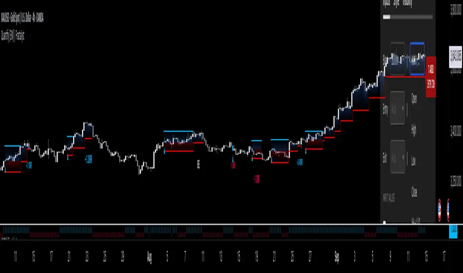
Stocks & Options P/L TrackerOverview:
The Stocks & Options P/L Tracker is a custom TradingView indicator developed to offer traders precise tracking of stocks & options trades’ profit and loss in real-time. It features a detailed display of P/L intervals, stop-loss and take-profit levels, and an adaptable trailing stop mechanism to help traders manage risk and optimize their trading strategies. This tool is particularly useful for active traders who seek immediate visual feedback on their trades’ performance.
Key Features:
Real-Time P/L Display: Computes and displays the P/L per contract/share and total P/L dynamically on the chart based on the specified entry price, relative to the current market price, and number of contracts or shares.
Configurable Take Profit and Stop Loss: Users can set take-profit and stop-loss amounts, and the indicator will visually mark these levels with corresponding dollar amounts for easy reference.
Trailing Stop Functionality: Offers an option to enable a trailing stop that automatically adjusts based on price movements.
Interval-Based P/L Tracking: Uses customizable intervals to display projected P/L levels above and below the entry price, helping users understand potential profit or loss scenarios at a glance.
Dynamic Labeling and Alerts: Visual labels are used to mark P/L, take-profit, stop-loss, trailing stop, and entry levels. These labels update dynamically on each new price bar to provide immediate insights into trade performance. NOTE: Due to TradingView's limitations with server-side alerts on fixed prices, dynamic alerts (for Take Profit, Stop Loss, and Trailing Stop) that adjust with price changes are not yet available. Alerts must be manually reset to your desired price each time.
Clean and Responsive Design: Utilizes color-coded labels and lines for P/L intervals, making it easy to distinguish profit, loss, stop, and take-profit zones. Colors adjust automatically to the current price to maintain clarity.
User Input Validation: Ensures appropriate input values for items like entry price, contract/share size, and profit/loss intervals to prevent errors and optimize performance.
Efficient Object Management: Implements object reusability for lines and labels to stay within Pine Script's object limits, ensuring smooth operation and maximum accuracy in real-time tracking.
Automatic Adjustments Based on Market Changes: Calculates and adjusts trailing stop levels dynamically based on highest price movement, which provides traders flexibility while maintaining risk controls.
Trader Benefits:
This indicator empowers traders with a robust tool to manage their trades visually and strategically on TradingView. The real-time feedback and customization options help traders make informed decisions, minimize risks, and maximize potential profits.
Happy Trading! :)
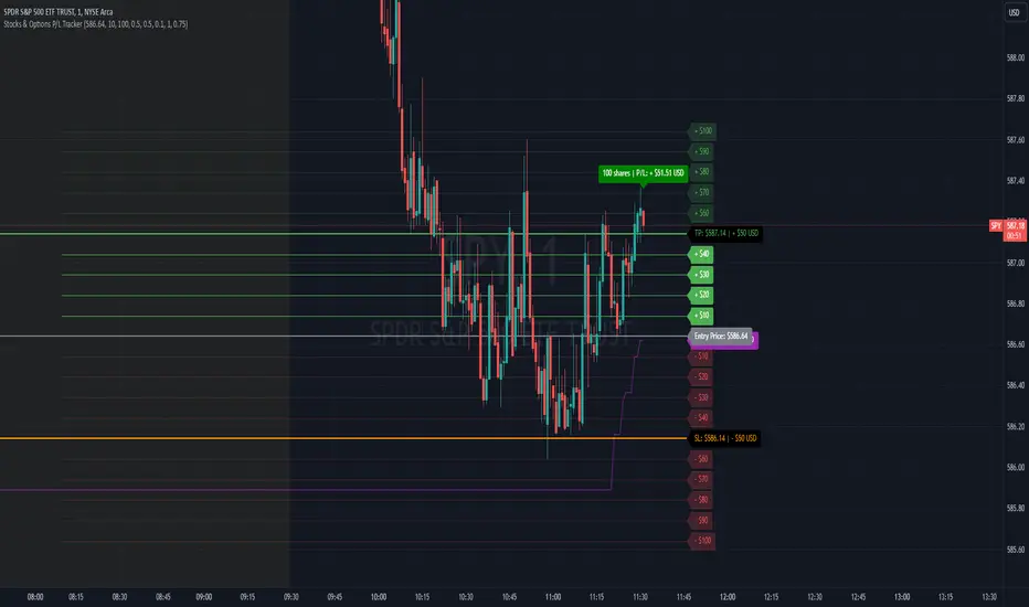
TS CalculatorWhat is Trailing Stop?
A trailing stop is a type of stop-loss order that adjusts itself as the price of an asset moves in a favorable direction. It’s designed to lock in profits or limit losses by following the asset’s price movement. Here’s how it works:
How a Trailing Stop Works
Initial Setup: You set a trailing stop at a certain percentage or dollar amount below (for long trades) or above (for short trades) the current market price.
Price Movement: As the price moves in your favor, the trailing stop moves with it, maintaining the set distance.
Locking in Profits: If the price reverses direction by the set amount, the trailing stop triggers a market order to sell (for long trades) or buy (for short trades), locking in your profits or limiting your losses.
Example
Long Trade: If you buy a stock at $100 and set a trailing stop at 10%, the stop-loss order will initially be at $90. If the stock price rises to $120, the trailing stop moves up to $108 (10% below $120). If the price then drops to $108, the trailing stop triggers a sell order.
Short Trade: If you short a stock at $100 and set a trailing stop at 10%, the stop-loss order will initially be at $110. If the stock price falls to $80, the trailing stop moves down to $88 (10% above $80). If the price then rises to $88, the trailing stop triggers a buy order.
Benefits
Automated Risk Management: It helps manage risk without the need to constantly monitor the market.
Profit Protection: It locks in profits as the price moves in your favor.
Flexibility: It adjusts dynamically with the market price, unlike a fixed stop-loss order.
What this script does ?
This script plots the Trailing Stop from the point of entry to current date, until it hits the trailing stop. Some of the market did not give the trailing stop values exactly so this script may give you a wise view of that.
Variables
Date : Date with YYYY-MM-DD format
Time : Time with HH:MM:SS format
Entry Price : Activation Price of TS order
Bounceback Ratio : Ratio for TS
Order Type : Position of order as Long/Short
There is an also a table implemented which shows
Entry
Ratio
Position
Current Stop
For possible updates feel free to contact me via DM.

Configurable Level Trading StrategyThe Dynamic Level Reversal Strategy is a trading approach designed to capitalize on price movements between key support and resistance levels. This strategy leverages configurable levels the trader determines, allowing for flexibility and adaptation to different market conditions.
Key Features:
Configurable Levels:
The strategy uses three key levels: Level 1 (Support), Level 2 (Middle), and Level 3 (Resistance). These levels can be adjusted directly within the script settings, making the strategy adaptable to various trading scenarios.
Buy and Sell Signals:
A buy signal is triggered when the price touches Level 1 and shows signs of reversal. The trader enters a position and sets an initial stop-loss just below Level 1.
As the price moves upward, the stop-loss is dynamically adjusted to just below Level 2 and Level 3, locking in profits while managing risk.
A sell signal is generated if the price reverses and crosses below the current stop-loss level, ensuring the trader exits the position with minimized losses.
Iterative Process:
The strategy allows for iterative trades, where the trader re-enters positions at Level 1 or Level 2 if the price revisits these levels, continually adjusting stop-losses and take-profit targets as the price oscillates between the defined levels.
Ideal Use Cases:
Range-Bound Markets: The strategy is particularly effective in markets where the price tends to oscillate between well-defined support and resistance levels.
Volatile Markets: The dynamic adjustment of stop-loss levels helps protect against sudden price reversals, making it suitable for volatile market conditions.
How to Use:
Set the desired levels (Level 1, Level 2, Level 3) based on your market analysis.
The script will automatically generate buy and sell signals, and adjust stop-loss levels as the price moves through the levels.
Monitor the signals and execute trades according to the strategy's guidelines.
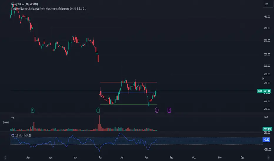
SL ManagerSTOP LOSS MANAGER
Overview:
The "SL Manager" indicator is designed to assist traders in managing their stop loss (SL) and take profit (TP) levels for both long and short positions. This tool helps you visualize intermediate levels, enhancing your trading decisions by providing crucial information on the chart.
Usage:
This indicator is particularly useful for traders who want to manage their trades more effectively by visualizing potential adjustment points for their stop loss and take profit levels. It helps in making informed decisions to maximize profits and minimize risks by providing clear levels to take partial profits and adjust stop losses.
Features:
Position Input: Select between "long" and "short" positions.
Entry Price: Specify the entry price of your trade.
Take Profit: Define the price level at which you want to take profit.
Stop Loss: Set the stop loss price level to manage your risk.
Intermediate Levels:
For both long and short positions, the indicator calculates and plots the following intermediate levels:
50% Take Profit (TP 50%): Midway between the entry price and the take profit level, where you can take partial profits and move your SL up to the 25% mark.
75% Take Profit (TP 75%): Three-quarters of the way from the entry price to the take profit level, where you can take partial profits and move your SL to breakeven.
Stop Loss Move to 25% (SL Move to 25%): A level where the stop loss can be adjusted to lock in profits.
Visualization:
The indicator plots the calculated levels directly on the chart, provided the data for the current day is available. Different color codes and line styles distinguish between the various levels:
TP 50% and TP 75% are plotted in green.
SL Move to 25% is plotted in red .
Entry/Breakeven is plotted in blue.

KillZones + ACD Fisher [TradingFinder] Sessions + Reversal Level🔵 Introduction
🟣 ACD Method
"The Logical Trader" opens with a thorough exploration of the ACD Methodology, which focuses on pinpointing particular price levels associated with the opening range.
This approach enables traders to establish reference points for their trades, using "A" and "C" points as entry markers. Additionally, the book covers the concept of the "Pivot Range" and how integrating it with the ACD method can help maximize position size while minimizing risk.
🟣 Session
The forex market is operational 24 hours a day, five days a week, closing only on Saturdays and Sundays. Typically, traders prefer to concentrate on one specific forex trading session rather than attempting to trade around the clock.
Trading sessions are defined time periods when a particular financial market is active, allowing for the execution of trades.
The most crucial trading sessions within the 24-hour cycle are the Asia, London, and New York sessions, as these are when substantial money flows and liquidity enter the market.
🟣 Kill Zone
Traders in financial markets earn profits by capitalizing on the difference between their buy/sell prices and the prevailing market prices.
Traders vary in their trading timelines.Some traders engage in daily or even hourly trading, necessitating activity during periods with optimal trading volumes and notable price movements.
Kill zones refer to parts of a session characterized by higher trading volumes and increased price volatility compared to the rest of the session.
🔵 How to Use
🟣 Session Times
The "Asia Session" comprises two parts: "Sydney" and "Tokyo." This session begins at 23:00 and ends at 06:00 UTC. The "Asia KillZone" starts at 23:00 and ends at 03:55 UTC.
The "London Session" includes "Frankfurt" and "London," starting at 07:00 and ending at 14:25 UTC. The "London KillZone" runs from 07:00 to 09:55 UTC.
The "New York" session starts at 14:30 and ends at 19:25 UTC, with the "New York am KillZone" beginning at 14:30 and ending at 22:55 UTC.
🟣 ACD Methodology
The ACD strategy is versatile, applicable to various markets such as stocks, commodities, and forex, providing clear buy and sell signals to set price targets and stop losses.
This strategy operates on the premise that the opening range of trades holds statistical significance daily, suggesting that initial market movements impact the market's behavior throughout the day.
Known as a breakout strategy, the ACD method thrives in volatile or strongly trending markets like crude oil and stocks.
Some key rules for employing the ACD strategy include :
Utilize points A and C as critical reference points, continually monitoring these during trades as they act as entry and exit markers.
Analyze daily and multi-day pivot ranges to understand market trends. Prices above the pivots indicate an upward trend, while prices below signal a downward trend.
In forex trading, the ACD strategy can be implemented using the ACD indicator, a technical tool that gauges the market's supply and demand balance. By evaluating trading volume and price, this indicator assists traders in identifying trend strength and optimal entry and exit points.
To effectively use the ACD indicator, consider the following :
Identifying robust trends: The ACD indicator can help pinpoint strong, consistent market trends.
Determining entry and exit points: ACD generates buy and sell signals to optimize trade timing.
Bullish Setup :
When the "A up" line is breached, it’s wise to wait briefly to confirm it’s not a "Fake Breakout" and that the price stabilizes above this line.
Upon entering the trade, the most effective stop loss is positioned below the "A down" line. It's advisable to backtest this to ensure the best outcomes. The recommended reward-to-risk ratio for this strategy is 1, which should also be verified through backtesting.
Bearish Setup :
When the "A down" line is breached, it’s prudent to wait briefly to ensure it’s not a "Fake Breakout" and that the price stabilizes below this line.
Upon entering the trade, the most effective stop loss is positioned above the "A up" line. Backtesting is recommended to confirm the best results. The recommended reward-to-risk ratio for this strategy is 1, which should also be validated through backtesting.
Advantages of Combining Kill Zone and ACD Method in Market Analysis :
Precise Trade Timing : Integrating the Kill Zone strategy with the ACD Method enhances precision in trade entries and exits. The ACD Method identifies key points for trading, while the Kill Zone focuses on high-activity periods, together ensuring optimal timing for trades.
Better Trend Identification : The ACD Method’s pivot ranges help spot market trends, and when combined with the Kill Zone’s emphasis on periods of significant price movement, traders can more effectively identify and follow strong market trends.
Maximized Profits and Minimized Risks : The ACD Method's structured approach to setting price targets and stop losses, coupled with the Kill Zone's high-volume trading periods, helps maximize profit potential while reducing risk.
Robust Risk Management : Combining these methods provides a comprehensive risk management strategy, strategically placing stop losses and protecting capital during volatile periods.
Versatility Across Markets : Both methods are applicable to various markets, including stocks, commodities, and forex, offering flexibility and adaptability in different trading environments.
Enhanced Confidence : Using the combined insights of the Kill Zone and ACD Method, traders gain confidence in their decision-making process, reducing emotional trading and improving consistency.
By merging the Kill Zone’s focus on trading volumes and the ACD Method’s structured breakout strategy, traders benefit from a synergistic approach that enhances precision, trend identification, and risk management across multiple markets.
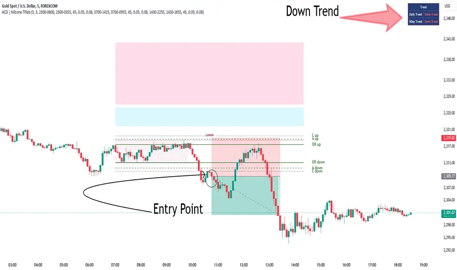
Quantum Duality Predictive Ranges### Quantum Duality Predictive Ranges v1.0
This Pine Script is designed to help traders predict price ranges and manage risk dynamically using ATR (Average True Range) calculations. It offers customizable settings, visual indicators, and alerts to assist in identifying trading opportunities and managing risk.
#### Key Features
- **Dynamic Risk Management**: Adjusts risk based on signals and cumulative risk.
- **Predictive Ranges**: Calculates predictive ranges based on ATR and user-defined multipliers.
- **Visual Indicators**: Plots lines and labels for easy visualization of trading signals and risk levels.
- **Alerts and Table**: Provides alerts for trading signals and displays a table with relevant trading data.
#### User Inputs
**EA Account Settings**
- **Initial Risk fixed in USD $**: Sets the initial risk amount in USD (default: 18).
- **Signal Multiply Factor for Risk**: Multiplier for signal risk (default: 1.257).
- **Pair Decimals**: Decimal places for pair pricing (default: 2).
**Trade Settings**
- **ATR Length**: Length for ATR calculation (default: 198).
- **ATR Factor**: Multiplier for ATR (default: 6.0).
- **ATR Source**: Source for ATR calculation (default: close).
- **ATR Multiplier**: Multiplier for defining RANGE Top/Bottom Levels (default: 0.45).
- **Inner Range Multiplier**: Multiplier for defining TP1 (default: 2.01).
- **Outer Range Multiplier**: Multiplier for defining TP2 (default: 3.0).
- **Spans Multiplier**: Multiplier for defining SL (default: 0.36).
**Display Options**
- **Display Table**: Option to display a table (default: true).
- **Display Labels for potential Gain and Loss**: Option to display gain/loss labels (default: true).
- **Display Labels for Bar counts since current Range**: Option to display bar counts (default: true).
- **Display Labels for Signals**: Option to display signal labels (default: true).
- **Line Width**: Width of the lines plotted (default: 1).
- **Line Transparency**: Transparency of the lines (default: 10).
- **Fill Transparency**: Transparency of the fill between lines (default: 75).
#### How It Works
1. **Predictive Ranges Calculation**:
- Calculates predictive ranges based on ATR, holds ATR values, and updates average values when price crosses defined levels.
2. **Risk Management and Signal Logic**:
- Counts the number of signals.
- Calculates cumulative and total risk based on signals.
- Resets signals and risk when price crosses predictive ranges.
3. **Entry Points and Potential Gains/Losses**:
- Determines buy and sell entry points.
- Calculates potential gains and losses for both buy and sell signals.
- Resets values when a new average range is established.
4. **Plotting and Alerts**:
- Plots lines for predictive ranges, spans, and stop loss levels.
- Displays labels for signals and potential gains/losses.
- Provides alerts for buy and sell signals with defined take profit and stop loss levels.
5. **Custom Ticker**:
- Renames tickers based on predefined rules (e.g., SPX500USD to SPX500).
#### Usage
1. **Set Up**:
- Adjust the input parameters in the settings menu to match your trading preferences and risk management strategy.
2. **Visualize**:
- View the plotted lines and labels on the chart to identify potential trading signals and manage risk.
3. **Alerts**:
- Enable alerts to receive notifications for buy and sell signals.
4. **Table**:
- Use the table to see a summary of important trading data, such as total risk and target levels.
This script provides a robust framework for managing risk and identifying trading opportunities using predictive ranges based on ATR. Happy trading!
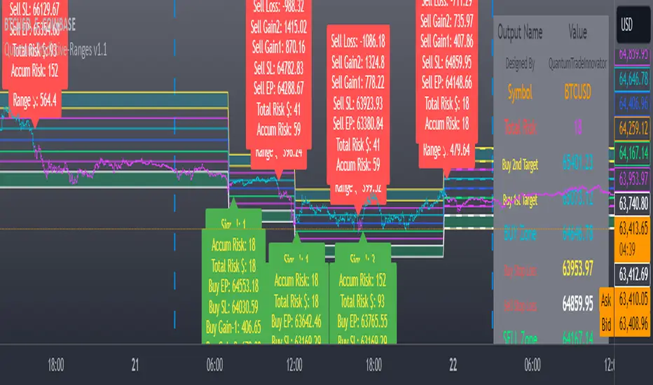
MetaFOX DCA (ASAP-RSI-BB%B-TV)Welcome To ' MetaFOX DCA (ASAP-RSI-BB%B-TV) ' Indicator.
This is not a Buy/Sell signals indicator, this is an indicator to help you create your own strategy using a variety of technical analyzing options within the indicator settings with the ability to do DCA (Dollar Cost Average) with up to 100 safety orders.
It is important when backtesting to get a real results, but this is impossible, especially when the time frame is large, because we don't know the real price action inside each candle, as we don't know whether the price reached the high or low first. but what I can say is that I present to you a backtest results in the worst possible case, meaning that if the same chart is repeated during the next period and you traded for the same period and with the same settings, the real results will be either identical to the results in the indicator or better (not worst). There will be no other factors except the slippage in the price when executing orders in the real trading, So I created a feature for that to increase the accuracy rate of the results. For more information, read this description.
Below I will explain all the properties and settings of the indicator:
A) 'Buy Strategies' Section: Your choices of strategies to Start a new trade: (All the conditions works as (And) not (OR), You have to choose one at least and you can choose more than one).
- 'ASAP (New Candle)': Start a trade as soon as possible at the opening of a new candle after exiting the previous trade.
- 'RSI': Using RSI as a technical analysis condition to start a trade.
- 'BB %B': Using BB %B as a technical analysis condition to start a trade.
- 'TV': Using tradingview crypto screener as a technical analysis condition to start a trade.
B) 'Exit Strategies' Section: Your choices of strategies to Exit the trades: (All the conditions works as (And) not (OR), You can choose more than one, But if you don't want to use any of them you have to activate the 'Use TP:' at least).
- 'ASAP (New Candle)': Exit a trade as soon as possible at the opening of a new candle after opening the previous trade.
- 'RSI': Using RSI as a technical analysis condition to exit a trade.
- 'BB %B': Using BB %B as a technical analysis condition to exit a trade.
- 'TV': Using tradingview crypto screener as a technical analysis condition to exit a trade.
C) 'Main Settings' Section:
- 'Trading Fees %': The Exchange trading fees in percentage (trading Commission).
- 'Entry Price Slippage %': Since real trading differs from backtest calculations, while in backtest results are calculated based on the open price of the candle, but in real trading there is a slippage from the open price of the candle resulting from the supply and demand in the real time trading, so this feature is to determine the slippage Which you think it is appropriate, then the entry prices of the trades will calculated higher than the open price of the start candle by the percentage of slippage that you set. If you don't want to calculate any slippage, just set it to zero, but I don't recommend that if you want the most realistic results.
Note: If (open price + slippage) is higher than the high of the candle then don't worry, I've kept this in consideration.
- 'Use SL': Activate to use stop loss percentage.
- 'SL %': Stop loss percentage.
- 'SL settings options box':
'SL From Base Price': Calculate the SL from the base order price (from the trade first entry price).
'SL From Avg. Price': Calculate the SL from the average price in case you use safety orders.
'SL From Last SO.': Calculate the SL from the last (lowest) safety order deviation.
ex: If you choose 'SL From Avg. Price' and SL% is 5, then the SL will be lower than the average price by 5% (in this case your SL will be dynamic until the price reaches all the safety orders unlike the other two SL options).
Note: This indicator programmed to be compatible with '3COMMAS' platform, but I added more options that came to my mind.
'3COMMAS' DCA bots uses 'SL From Base Price'.
- 'Use TP': Activate to use take profit percentage.
- 'TP %': Take profit percentage.
- 'Pure TP,SL': This feature was created due to the differences in the method of calculations between API tools trading platforms:
If the feature is not activated and (for example) the TP is 5%, this means that the price must move upward by only 5%, but you will not achieve a net profit of 5% due to the trading fees. but If the feature is activated, this means that you will get a net profit of 5%, and this means that the price must move upward by (5% for the TP + the equivalent of trading fees). The same idea is applied to the SL.
Note: '3COMMAS' DCA bots uses activated 'Pure TP,SL'.
- 'SO. Price Deviation %': Determines the decline percentage for the first safety order from the trade start entry price.
- 'SO. Step Scale': Determines the deviation multiplier for the safety orders.
Note: I'm using the same method of calculations for SO. (safety orders) levels that '3COMMAS' platform is using. If there is any difference between the '3COMMAS' calculations and the platform that you are using, please let me know.
'3COMMAS' DCA bots minimum 'SO. Price Deviation %' is (0.21)
'3COMMAS' DCA bots minimum 'SO. Step Scale' is (0.1)
- 'SO. Volume Scale': Determines the base order size multiplier for the safety orders sizes.
ex: If you used 10$ to buy at the trade start (base order size) and your 'SO. Volume Scale' is 2, then the 1st SO. size will be 20, the 2nd SO. size will be 40 and so on.
- 'SO. Count': Determines the number of safety orders that you want. If you want to trade without safety orders set it to zero.
'3COMMAS' DCA bots minimum 'SO. Volume Scale' is (0.1)
- 'Exchange Min. Size': The exchange minimum size per trade, It's important to prevent you from setting the base order Size less than the exchange limit. It's also important for the backtest results calculations.
ex: If you setup your strategy settings and it led to a loss to the point that you can't trade any more due to insufficient funds and your base order size share from the strategy becomes less than the exchange minimum trade size, then the indicator will show you a warning and will show you the point where you stopped the trading (It works in compatible with the initial capital). I recommend to set it a little bit higher than the real exchange minimum trade size especially if you trade without safety orders to not stuck in the trade if you hit the stop loss
- 'BO. Size': The base order size (funds you use at the trade entry).
- 'Initial Capital': The total funds allocated for trading using your strategy settings, It can be more than what is required in the strategy to cover the deficit in case of a loss, but it should not exceed the funds that you actually have for trading using this strategy settings, It's important to prevent you from setting up a strategy which requires funds more than what you have. It's also has other important benefits (refer to 'Exchange Min. Size' for more information).
- 'Accumulative Results': This feature is also called re-invest profits & risk reduction. If it's not activated then you will use the same funds size in each new trade whether you are in profit or loss till the (initial capitals + net results) turns insufficient. If it's activated then you will reuse your profits and losses in each new trade.
ex: The feature is active and your first trade ended with a net profit of 1000$, the next trade will add the 1000$ to the trade funds size and it will be distributed as a percentage to the BO. & SO.s according to your strategy settings. The same idea in case of a loss, the trade funds size will be reduced.
D) 'RSI Strategy' Section:
- 'Buy': RSI technical condition to start a trade. Has no effect if you don't choose 'RSI' option in 'Buy Strategies'.
- 'Exit': RSI technical condition to exit a trade. Has no effect if you don't choose 'RSI' option in 'Exit Strategies'.
E) 'TV Strategy' Section:
- 'Buy': TradingView Crypto Screener technical condition to start a trade. Has no effect if you don't choose 'TV' option in 'Buy Strategies'.
- 'Exit': TradingView Crypto Screener technical condition to exit a trade. Has no effect if you don't choose 'TV' option in 'Exit Strategies'.
F) 'BB %B Strategy' Section:
- 'Buy': BB %B technical condition to start a trade. Has no effect if you don't choose 'BB %B' option in 'Buy Strategies'.
- 'Exit': BB %B technical condition to exit a trade. Has no effect if you don't choose 'BB %B' option in 'Exit Strategies'.
G) 'Plot' Section:
- 'Signals': Plots buy and exit signals.
- 'BO': Plots the trade entry price (base order price).
- 'AVG': Plots the trade average price.
- 'AVG options box': Your choice to plot the trade average price type:
'Avg. With Fees': The trade average price including the trading fees, If you exit the trade at this price the trade net profit will be 0.00
'Avg. Without Fees': The trade average price but not including the trading fees, If you exit the trade at this price the trade net profit will be a loss equivalent to the trading fees.
- 'TP': Plots the trade take profit price.
- 'SL': Plots the trade stop loss price.
- 'Last SO': Plots the trade last safety order that the price reached.
- 'Exit Price': Plots a mark on the trade exit price, It plots in 3 colors as below:
Red (Default): Trade exit at a loss.
Green (Default): Trade exit at a profit.
Yellow (Default): Trade exit at a profit but this is a special case where we have to calculate the profits before reaching the safety orders (if any) on that candle (compatible with the idea of getting strategy results at the worst case).
- 'Result Table': Plots your strategy result table. The net profit percentage shown is a percentage of the 'initial capital'.
- 'TA Values': Plots your used strategies Technical analysis values. (Green cells means valid condition).
- 'Help Table': Plots a table to help you discover 100 safety orders with its deviations and the total funds needed for your strategy settings. Deviations shown in red is impossible to use because its price is <= 0.00
- 'Portfolio Chart': Plots your Portfolio status during the entire trading period in addition to the highest and lowest level reached. It's important when evaluating any strategy not only to look at the final result, but also to look at the change in results over the entire trading period. Perhaps the results were worryingly negative at some point before they rose again and made a profit. This feature helps you to see the whole picture.
- 'Welcome Message': Plots a welcome message and showing you the idea behind this indicator.
- 'Green Net Profit %': It plots the 'Net Profit %' in the result table in green color if the result is equal to or above the value that you entered.
- 'Green Win Rate %': It plots the 'Win Rate %' in the result table in green color if the result is equal to or above the value that you entered.
- 'User Notes Area': An empty text area, Feel free to use this area to write your notes so you don't forget them.
The indicator will take care of you. In some cases, warning messages will appear for you. Read them carefully, as they mean that you have done an illogical error in the indicator settings. Also, the indicator will sometimes stop working for the same reason mentioned above. If that happens then click on the red (!) next to the indicator name and read the message to find out what illogical error you have done.
Please enjoy the indicator and let me know your thoughts in the comments below.

EMA Envelope - Signal with Stoploss and Takeprofit LevelsDescription:
This Pine Script indicator implements the EMA Envelope strategy, which utilizes Exponential Moving Averages (EMA) to create an envelope around the price chart. The strategy generates buy and sell signals based on the crossing of the price above and below the upper and lower EMA envelopes, respectively. It also incorporates additional features such as stop-loss and take-profit levels for risk management.
Indicator Settings:
EMA Length: Specifies the period for the short-term Exponential Moving Average.
Long Term EMA Length: Defines the period for the long-term Exponential Moving Average used for signal filtering.
Take Profit Ratio: Determines the ratio for calculating the take-profit levels based on the stop-loss.
Filter Signal on Long Term EMA: Enables or disables the filtering of buy/sell signals using the long-term EMA.
Show only recent signal: When enabled, shows only the most recent buy/sell signals.
Buy and Sell Signals:
The indicator generates buy signals when the price crosses above the upper EMA envelope and the previous low was below the upper EMA envelope. Additionally, you can choose to filter buy signals based on whether the closing price is above the long-term EMA.
Conversely, sell signals are generated when the price crosses below the lower EMA envelope, and the previous high was above the lower EMA envelope. Similar to buy signals, sell signals can also be filtered using the long-term EMA.
Note: Signal works well on Higher Timeframes like Daily/8hrs/4hrs/1hr.
Stop-Loss and Take-Profit Levels:
For buy signals, the stop-loss is set at the lower EMA level, while the take-profit level is calculated by adding a specified ratio of the difference between the low and the stop-loss level to the low price.
For sell signals, the stop-loss is set at the upper EMA level, and the take-profit level is calculated by subtracting a specified ratio of the difference between the stop-loss level and the high price from the high price.
Disclaimer:
This indicator is provided for educational and informational purposes only. Trading involves significant risk, and past performance does not guarantee future results. Users are solely responsible for their trading decisions and should conduct their own research and risk management. The author shall not be held liable for any losses or damages arising from the use of this indicator.
Note: Always test the indicator thoroughly on historical data and consider paper trading before applying it to live trading environments.

GKD-M Baseline Optimizer [Loxx]Giga Kaleidoscope GKD-M Baseline Optimizer is a Metamorphosis module included in Loxx's "Giga Kaleidoscope Modularized Trading System".
The Baseline Optimizer enables traders to backtest over 60 moving averages using variable period inputs. It then exports the baseline with the highest cumulative win rate per candle to any baseline-enabled GKD backtest. To perform the backtesting, the trader selects an initial period input (default is 60) and a skip value that increments the initial period input up to seven times. For instance, if a skip value of 5 is chosen, the Baseline Optimizer will run the backtest for the selected moving average on periods such as 60, 65, 70, 75, and so on, up to 90. If the user selects an initial period input of 45 and a skip value of 2, the Baseline Optimizer will conduct backtests for the chosen moving average on periods like 45, 47, 49, 51, and so forth, up to 57.
The Baseline Optimizer provides a table displaying the output of the backtests for a specified date range. The table output represents the cumulative win rate for the given date range.
On the Metamorphosis side of the Baseline Optimizer, a cumulative backtest is calculated for each candle within the date range. This means that each candle may exhibit a different distribution of period inputs with the highest win rate for a particular moving average. The Baseline Optimizer identifies the period input combination with the highest win rates for long and short positions and creates a win-rate adaptive long and short moving average chart. The moving average used for shorts differs from the moving average used for longs, and the moving average for each candle may vary from any other candle. This customized baseline can then be exported to all baseline-enabled GKD backtests.
The backtest employed in the Baseline Optimizer is a Solo Confirmation Simple, allowing only one take profit and one stop loss to be set.
Lastly, the Baseline Optimizer incorporates Goldie Locks Zone filtering, which can be utilized for signal generation in advanced GKD backtests.
█ Moving Averages included in the Baseline Optimizer
Adaptive Moving Average - AMA
ADXvma - Average Directional Volatility Moving Average
Ahrens Moving Average
Alexander Moving Average - ALXMA
Deviation Scaled Moving Average - DSMA
Donchian
Double Exponential Moving Average - DEMA
Double Smoothed Exponential Moving Average - DSEMA
Double Smoothed FEMA - DSFEMA
Double Smoothed Range Weighted EMA - DSRWEMA
Double Smoothed Wilders EMA - DSWEMA
Double Weighted Moving Average - DWMA
Exponential Moving Average - EMA
Fast Exponential Moving Average - FEMA
Fractal Adaptive Moving Average - FRAMA
Generalized DEMA - GDEMA
Generalized Double DEMA - GDDEMA
Hull Moving Average (Type 1) - HMA1
Hull Moving Average (Type 2) - HMA2
Hull Moving Average (Type 3) - HMA3
Hull Moving Average (Type 4) - HMA4
IE /2 - Early T3 by Tim Tilson
Integral of Linear Regression Slope - ILRS
Kaufman Adaptive Moving Average - KAMA
Leader Exponential Moving Average
Linear Regression Value - LSMA ( Least Squares Moving Average )
Linear Weighted Moving Average - LWMA
McGinley Dynamic
McNicholl EMA
Non-Lag Moving Average
Ocean NMA Moving Average - ONMAMA
One More Moving Average - OMA
Parabolic Weighted Moving Average
Probability Density Function Moving Average - PDFMA
Quadratic Regression Moving Average - QRMA
Regularized EMA - REMA
Range Weighted EMA - RWEMA
Recursive Moving Trendline
Simple Decycler - SDEC
Simple Jurik Moving Average - SJMA
Simple Moving Average - SMA
Sine Weighted Moving Average
Smoothed LWMA - SLWMA
Smoothed Moving Average - SMMA
Smoother
Super Smoother
T3
Three-pole Ehlers Butterworth
Three-pole Ehlers Smoother
Triangular Moving Average - TMA
Triple Exponential Moving Average - TEMA
Two-pole Ehlers Butterworth
Two-pole Ehlers smoother
Variable Index Dynamic Average - VIDYA
Variable Moving Average - VMA
Volume Weighted EMA - VEMA
Volume Weighted Moving Average - VWMA
Zero-Lag DEMA - Zero Lag Exponential Moving Average
Zero-Lag Moving Average
Zero Lag TEMA - Zero Lag Triple Exponential Moving Average
Adaptive Moving Average - AMA
The Adaptive Moving Average (AMA) is a moving average that changes its sensitivity to price moves depending on the calculated volatility. It becomes more sensitive during periods when the price is moving smoothly in a certain direction and becomes less sensitive when the price is volatile.
ADXvma - Average Directional Volatility Moving Average
Linnsoft's ADXvma formula is a volatility-based moving average, with the volatility being determined by the value of the ADX indicator.
The ADXvma has the SMA in Chande's CMO replaced with an EMA , it then uses a few more layers of EMA smoothing before the "Volatility Index" is calculated.
A side effect is, those additional layers slow down the ADXvma when you compare it to Chande's Variable Index Dynamic Average VIDYA .
The ADXVMA provides support during uptrends and resistance during downtrends and will stay flat for longer, but will create some of the most accurate market signals when it decides to move.
Ahrens Moving Average
Richard D. Ahrens's Moving Average promises "Smoother Data" that isn't influenced by the occasional price spike. It works by using the Open and the Close in his formula so that the only time the Ahrens Moving Average will change is when the candlestick is either making new highs or new lows.
Alexander Moving Average - ALXMA
This Moving Average uses an elaborate smoothing formula and utilizes a 7 period Moving Average. It corresponds to fitting a second-order polynomial to seven consecutive observations. This moving average is rarely used in trading but is interesting as this Moving Average has been applied to diffusion indexes that tend to be very volatile.
Deviation Scaled Moving Average - DSMA
The Deviation-Scaled Moving Average is a data smoothing technique that acts like an exponential moving average with a dynamic smoothing coefficient. The smoothing coefficient is automatically updated based on the magnitude of price changes. In the Deviation-Scaled Moving Average, the standard deviation from the mean is chosen to be the measure of this magnitude. The resulting indicator provides substantial smoothing of the data even when price changes are small while quickly adapting to these changes.
Donchian
Donchian Channels are three lines generated by moving average calculations that comprise an indicator formed by upper and lower bands around a midrange or median band. The upper band marks the highest price of a security over N periods while the lower band marks the lowest price of a security over N periods.
Double Exponential Moving Average - DEMA
The Double Exponential Moving Average ( DEMA ) combines a smoothed EMA and a single EMA to provide a low-lag indicator. It's primary purpose is to reduce the amount of "lagging entry" opportunities, and like all Moving Averages, the DEMA confirms uptrends whenever price crosses on top of it and closes above it, and confirms downtrends when the price crosses under it and closes below it - but with significantly less lag.
Double Smoothed Exponential Moving Average - DSEMA
The Double Smoothed Exponential Moving Average is a lot less laggy compared to a traditional EMA . It's also considered a leading indicator compared to the EMA , and is best utilized whenever smoothness and speed of reaction to market changes are required.
Double Smoothed FEMA - DSFEMA
Same as the Double Exponential Moving Average (DEMA), but uses a faster version of EMA for its calculation.
Double Smoothed Range Weighted EMA - DSRWEMA
Range weighted exponential moving average (EMA) is, unlike the "regular" range weighted average calculated in a different way. Even though the basis - the range weighting - is the same, the way how it is calculated is completely different. By definition this type of EMA is calculated as a ratio of EMA of price*weight / EMA of weight. And the results are very different and the two should be considered as completely different types of averages. The higher than EMA to price changes responsiveness when the ranges increase remains in this EMA too and in those cases this EMA is clearly leading the "regular" EMA. This version includes double smoothing.
Double Smoothed Wilders EMA - DSWEMA
Welles Wilder was frequently using one "special" case of EMA (Exponential Moving Average) that is due to that fact (that he used it) sometimes called Wilder's EMA. This version is adding double smoothing to Wilder's EMA in order to make it "faster" (it is more responsive to market prices than the original) and is still keeping very smooth values.
Double Weighted Moving Average - DWMA
Double weighted moving average is an LWMA (Linear Weighted Moving Average). Instead of doing one cycle for calculating the LWMA, the indicator is made to cycle the loop 2 times. That produces a smoother values than the original LWMA
Exponential Moving Average - EMA
The EMA places more significance on recent data points and moves closer to price than the SMA ( Simple Moving Average ). It reacts faster to volatility due to its emphasis on recent data and is known for its ability to give greater weight to recent and more relevant data. The EMA is therefore seen as an enhancement over the SMA .
Fast Exponential Moving Average - FEMA
An Exponential Moving Average with a short look-back period.
Fractal Adaptive Moving Average - FRAMA
The Fractal Adaptive Moving Average by John Ehlers is an intelligent adaptive Moving Average which takes the importance of price changes into account and follows price closely enough to display significant moves whilst remaining flat if price ranges. The FRAMA does this by dynamically adjusting the look-back period based on the market's fractal geometry.
Generalized DEMA - GDEMA
The double exponential moving average (DEMA), was developed by Patrick Mulloy in an attempt to reduce the amount of lag time found in traditional moving averages. It was first introduced in the February 1994 issue of the magazine Technical Analysis of Stocks & Commodities in Mulloy's article "Smoothing Data with Faster Moving Averages.". Instead of using fixed multiplication factor in the final DEMA formula, the generalized version allows you to change it. By varying the "volume factor" form 0 to 1 you apply different multiplications and thus producing DEMA with different "speed" - the higher the volume factor is the "faster" the DEMA will be (but also the slope of it will be less smooth). The volume factor is limited in the calculation to 1 since any volume factor that is larger than 1 is increasing the overshooting to the extent that some volume factors usage makes the indicator unusable.
Generalized Double DEMA - GDDEMA
The double exponential moving average (DEMA), was developed by Patrick Mulloy in an attempt to reduce the amount of lag time found in traditional moving averages. It was first introduced in the February 1994 issue of the magazine Technical Analysis of Stocks & Commodities in Mulloy's article "Smoothing Data with Faster Moving Averages''. This is an extension of the Generalized DEMA using Tim Tillsons (the inventor of T3) idea, and is using GDEMA of GDEMA for calculation (which is the "middle step" of T3 calculation). Since there are no versions showing that middle step, this version covers that too. The result is smoother than Generalized DEMA, but is less smooth than T3 - one has to do some experimenting in order to find the optimal way to use it, but in any case, since it is "faster" than the T3 (Tim Tillson T3) and still smooth, it looks like a good compromise between speed and smoothness.
Hull Moving Average (Type 1) - HMA1
Alan Hull's HMA makes use of weighted moving averages to prioritize recent values and greatly reduce lag whilst maintaining the smoothness of a traditional Moving Average. For this reason, it's seen as a well-suited Moving Average for identifying entry points. This version uses SMA for smoothing.
Hull Moving Average (Type 2) - HMA2
Alan Hull's HMA makes use of weighted moving averages to prioritize recent values and greatly reduce lag whilst maintaining the smoothness of a traditional Moving Average. For this reason, it's seen as a well-suited Moving Average for identifying entry points. This version uses EMA for smoothing.
Hull Moving Average (Type 3) - HMA3
Alan Hull's HMA makes use of weighted moving averages to prioritize recent values and greatly reduce lag whilst maintaining the smoothness of a traditional Moving Average. For this reason, it's seen as a well-suited Moving Average for identifying entry points. This version uses LWMA for smoothing.
Hull Moving Average (Type 4) - HMA4
Alan Hull's HMA makes use of weighted moving averages to prioritize recent values and greatly reduce lag whilst maintaining the smoothness of a traditional Moving Average. For this reason, it's seen as a well-suited Moving Average for identifying entry points. This version uses SMMA for smoothing.
IE /2 - Early T3 by Tim Tilson and T3 new
The T3 moving average is a type of technical indicator used in financial analysis to identify trends in price movements. It is similar to the Exponential Moving Average (EMA) and the Double Exponential Moving Average (DEMA), but uses a different smoothing algorithm.
The T3 moving average is calculated using a series of exponential moving averages that are designed to filter out noise and smooth the data. The resulting smoothed data is then weighted with a non-linear function to produce a final output that is more responsive to changes in trend direction.
The T3 moving average can be customized by adjusting the length of the moving average, as well as the weighting function used to smooth the data. It is commonly used in conjunction with other technical indicators as part of a larger trading strategy.
Integral of Linear Regression Slope - ILRS
A Moving Average where the slope of a linear regression line is simply integrated as it is fitted in a moving window of length N (natural numbers in maths) across the data. The derivative of ILRS is the linear regression slope. ILRS is not the same as a SMA ( Simple Moving Average ) of length N, which is actually the midpoint of the linear regression line as it moves across the data.
Kaufman Adaptive Moving Average - KAMA
Developed by Perry Kaufman, Kaufman's Adaptive Moving Average (KAMA) is a moving average designed to account for market noise or volatility. KAMA will closely follow prices when the price swings are relatively small and the noise is low.
Leader Exponential Moving Average
The Leader EMA was created by Giorgos E. Siligardos who created a Moving Average which was able to eliminate lag altogether whilst maintaining some smoothness. It was first described during his research paper "MACD Leader" where he applied this to the MACD to improve its signals and remove its lagging issue. This filter uses his leading MACD's "modified EMA" and can be used as a zero lag filter.
Linear Regression Value - LSMA ( Least Squares Moving Average )
LSMA as a Moving Average is based on plotting the end point of the linear regression line. It compares the current value to the prior value and a determination is made of a possible trend, eg. the linear regression line is pointing up or down.
Linear Weighted Moving Average - LWMA
LWMA reacts to price quicker than the SMA and EMA . Although it's similar to the Simple Moving Average , the difference is that a weight coefficient is multiplied to the price which means the most recent price has the highest weighting, and each prior price has progressively less weight. The weights drop in a linear fashion.
McGinley Dynamic
John McGinley created this Moving Average to track prices better than traditional Moving Averages. It does this by incorporating an automatic adjustment factor into its formula, which speeds (or slows) the indicator in trending, or ranging, markets.
McNicholl EMA
Dennis McNicholl developed this Moving Average to use as his center line for his "Better Bollinger Bands" indicator and was successful because it responded better to volatility changes over the standard SMA and managed to avoid common whipsaws.
Non-lag moving average
The Non Lag Moving average follows price closely and gives very quick signals as well as early signals of price change. As a standalone Moving Average, it should not be used on its own, but as an additional confluence tool for early signals.
Ocean NMA Moving Average - ONMAMA
Created by Jim Sloman, the NMA is a moving average that automatically adjusts to volatility without being programmed to do so. For more info, read his guide "Ocean Theory, an Introduction"
One More Moving Average (OMA)
The One More Moving Average (OMA) is a technical indicator that calculates a series of Jurik-style moving averages in order to reduce noise and provide smoother price data. It uses six exponential moving averages to generate the final value, with the length of the moving averages determined by an adaptive algorithm that adjusts to the current market conditions. The algorithm calculates the average period by comparing the signal to noise ratio and using this value to determine the length of the moving averages. The resulting values are used to generate the final value of the OMA, which can be used to identify trends and potential changes in trend direction.
Parabolic Weighted Moving Average
The Parabolic Weighted Moving Average is a variation of the Linear Weighted Moving Average . The Linear Weighted Moving Average calculates the average by assigning different weights to each element in its calculation. The Parabolic Weighted Moving Average is a variation that allows weights to be changed to form a parabolic curve. It is done simply by using the Power parameter of this indicator.
Probability Density Function Moving Average - PDFMA
Probability density function based MA is a sort of weighted moving average that uses probability density function to calculate the weights. By its nature it is similar to a lot of digital filters.
Quadratic Regression Moving Average - QRMA
A quadratic regression is the process of finding the equation of the parabola that best fits a set of data. This moving average is an obscure concept that was posted to Forex forums in around 2008.
Regularized EMA - REMA
The regularized exponential moving average (REMA) by Chris Satchwell is a variation on the EMA (see Exponential Moving Average) designed to be smoother but not introduce too much extra lag.
Range Weighted EMA - RWEMA
This indicator is a variation of the range weighted EMA. The variation comes from a possible need to make that indicator a bit less "noisy" when it comes to slope changes. The method used for calculating this variation is the method described by Lee Leibfarth in his article "Trading With An Adaptive Price Zone".
Recursive Moving Trendline
Dennis Meyers's Recursive Moving Trendline uses a recursive (repeated application of a rule) polynomial fit, a technique that uses a small number of past values estimations of price and today's price to predict tomorrow's price.
Simple Decycler - SDEC
The Ehlers Simple Decycler study is a virtually zero-lag technical indicator proposed by John F. Ehlers. The original idea behind this study (and several others created by John F. Ehlers) is that market data can be considered a continuum of cycle periods with different cycle amplitudes. Thus, trending periods can be considered segments of longer cycles, or, in other words, low-frequency segments. Applying the right filter might help identify these segments.
Simple Loxx Moving Average - SLMA
A three stage moving average combining an adaptive EMA, a Kalman Filter, and a Kauffman adaptive filter.
Simple Moving Average - SMA
The SMA calculates the average of a range of prices by adding recent prices and then dividing that figure by the number of time periods in the calculation average. It is the most basic Moving Average which is seen as a reliable tool for starting off with Moving Average studies. As reliable as it may be, the basic moving average will work better when it's enhanced into an EMA .
Sine Weighted Moving Average
The Sine Weighted Moving Average assigns the most weight at the middle of the data set. It does this by weighting from the first half of a Sine Wave Cycle and the most weighting is given to the data in the middle of that data set. The Sine WMA closely resembles the TMA (Triangular Moving Average).
Smoothed LWMA - SLWMA
A smoothed version of the LWMA
Smoothed Moving Average - SMMA
The Smoothed Moving Average is similar to the Simple Moving Average ( SMA ), but aims to reduce noise rather than reduce lag. SMMA takes all prices into account and uses a long lookback period. Due to this, it's seen as an accurate yet laggy Moving Average.
Smoother
The Smoother filter is a faster-reacting smoothing technique which generates considerably less lag than the SMMA ( Smoothed Moving Average ). It gives earlier signals but can also create false signals due to its earlier reactions. This filter is sometimes wrongly mistaken for the superior Jurik Smoothing algorithm.
Super Smoother
The Super Smoother filter uses John Ehlers’s “Super Smoother” which consists of a Two pole Butterworth filter combined with a 2-bar SMA ( Simple Moving Average ) that suppresses the 22050 Hz Nyquist frequency: A characteristic of a sampler, which converts a continuous function or signal into a discrete sequence.
Three-pole Ehlers Butterworth
The 3 pole Ehlers Butterworth (as well as the Two pole Butterworth) are both superior alternatives to the EMA and SMA . They aim at producing less lag whilst maintaining accuracy. The 2 pole filter will give you a better approximation for price, whereas the 3 pole filter has superior smoothing.
Three-pole Ehlers smoother
The 3 pole Ehlers smoother works almost as close to price as the above mentioned 3 Pole Ehlers Butterworth. It acts as a strong baseline for signals but removes some noise. Side by side, it hardly differs from the Three Pole Ehlers Butterworth but when examined closely, it has better overshoot reduction compared to the 3 pole Ehlers Butterworth.
Triangular Moving Average - TMA
The TMA is similar to the EMA but uses a different weighting scheme. Exponential and weighted Moving Averages will assign weight to the most recent price data. Simple moving averages will assign the weight equally across all the price data. With a TMA (Triangular Moving Average), it is double smoother (averaged twice) so the majority of the weight is assigned to the middle portion of the data.
Triple Exponential Moving Average - TEMA
The TEMA uses multiple EMA calculations as well as subtracting lag to create a tool which can be used for scalping pullbacks. As it follows price closely, its signals are considered very noisy and should only be used in extremely fast-paced trading conditions.
Two-pole Ehlers Butterworth
The 2 pole Ehlers Butterworth (as well as the three pole Butterworth mentioned above) is another filter that cuts out the noise and follows the price closely. The 2 pole is seen as a faster, leading filter over the 3 pole and follows price a bit more closely. Analysts will utilize both a 2 pole and a 3 pole Butterworth on the same chart using the same period, but having both on chart allows its crosses to be traded.
Two-pole Ehlers smoother
A smoother version of the Two pole Ehlers Butterworth. This filter is the faster version out of the 3 pole Ehlers Butterworth. It does a decent job at cutting out market noise whilst emphasizing a closer following to price over the 3 pole Ehlers .
Variable Index Dynamic Average - VIDYA
Variable Index Dynamic Average Technical Indicator ( VIDYA ) was developed by Tushar Chande. It is an original method of calculating the Exponential Moving Average ( EMA ) with the dynamically changing period of averaging.
Variable Moving Average - VMA
The Variable Moving Average (VMA) is a study that uses an Exponential Moving Average being able to automatically adjust its smoothing factor according to the market volatility.
Volume Weighted EMA - VEMA
An EMA that uses a volume and price weighted calculation instead of the standard price input.
Volume Weighted Moving Average - VWMA
A Volume Weighted Moving Average is a moving average where more weight is given to bars with heavy volume than with light volume. Thus the value of the moving average will be closer to where most trading actually happened than it otherwise would be without being volume weighted.
Zero-Lag DEMA - Zero Lag Double Exponential Moving Average
John Ehlers's Zero Lag DEMA's aim is to eliminate the inherent lag associated with all trend following indicators which average a price over time. Because this is a Double Exponential Moving Average with Zero Lag, it has a tendency to overshoot and create a lot of false signals for swing trading. It can however be used for quick scalping or as a secondary indicator for confluence.
Zero-Lag Moving Average
The Zero Lag Moving Average is described by its creator, John Ehlers , as a Moving Average with absolutely no delay. And it's for this reason that this filter will cause a lot of abrupt signals which will not be ideal for medium to long-term traders. This filter is designed to follow price as close as possible whilst de-lagging data instead of basing it on regular data. The way this is done is by attempting to remove the cumulative effect of the Moving Average.
Zero-Lag TEMA - Zero Lag Triple Exponential Moving Average
Just like the Zero Lag DEMA , this filter will give you the fastest signals out of all the Zero Lag Moving Averages. This is useful for scalping but dangerous for medium to long-term traders, especially during market Volatility and news events. Having no lag, this filter also has no smoothing in its signals and can cause some very bizarre behavior when applied to certain indicators.
█ Volatility Goldie Locks Zone
The Goldie Locks Zone volatility filter is the standard first-pass filter used in all advanced GKD backtests (Complex, Super Complex, and Full GKd). This filter requires the price to fall within a range determined by multiples of volatility. The Goldie Locks Zone is separate from the core Baseline and utilizes its own moving average with Loxx's Exotic Source Types you can read about below.
On the chart, you will find green and red dots positioned at the top, indicating whether a candle qualifies for a long or short trade respectively. Additionally, green and red triangles are located at the bottom of the chart, signifying whether the trigger has crossed up or down and qualifies within the Goldie Locks zone. The Goldie Locks zone is represented by a white color on the mean line, indicating low volatility levels that are not suitable for trading.
█ Volatility Types Included in the Baseline Optimizer
The GKD system utilizes volatility-based take profits and stop losses. Each take profit and stop loss is calculated as a multiple of volatility. Users can also adjust the multiplier values in the settings.
This module includes 17 types of volatility:
Close-to-Close
Parkinson
Garman-Klass
Rogers-Satchell
Yang-Zhang
Garman-Klass-Yang-Zhang
Exponential Weighted Moving Average
Standard Deviation of Log Returns
Pseudo GARCH(2,2)
Average True Range
True Range Double
Standard Deviation
Adaptive Deviation
Median Absolute Deviation
Efficiency-Ratio Adaptive ATR
Mean Absolute Deviation
Static Percent
Various volatility estimators and indicators that investors and traders can use to measure the dispersion or volatility of a financial instrument's price. Each estimator has its strengths and weaknesses, and the choice of estimator should depend on the specific needs and circumstances of the user.
Close-to-Close
Close-to-Close volatility is a classic and widely used volatility measure, sometimes referred to as historical volatility.
Volatility is an indicator of the speed of a stock price change. A stock with high volatility is one where the price changes rapidly and with a larger amplitude. The more volatile a stock is, the riskier it is.
Close-to-close historical volatility is calculated using only a stock's closing prices. It is the simplest volatility estimator. However, in many cases, it is not precise enough. Stock prices could jump significantly during a trading session and return to the opening value at the end. That means that a considerable amount of price information is not taken into account by close-to-close volatility.
Despite its drawbacks, Close-to-Close volatility is still useful in cases where the instrument doesn't have intraday prices. For example, mutual funds calculate their net asset values daily or weekly, and thus their prices are not suitable for more sophisticated volatility estimators.
Parkinson
Parkinson volatility is a volatility measure that uses the stock’s high and low price of the day.
The main difference between regular volatility and Parkinson volatility is that the latter uses high and low prices for a day, rather than only the closing price. This is useful as close-to-close prices could show little difference while large price movements could have occurred during the day. Thus, Parkinson's volatility is considered more precise and requires less data for calculation than close-to-close volatility.
One drawback of this estimator is that it doesn't take into account price movements after the market closes. Hence, it systematically undervalues volatility. This drawback is addressed in the Garman-Klass volatility estimator.
Garman-Klass
Garman-Klass is a volatility estimator that incorporates open, low, high, and close prices of a security.
Garman-Klass volatility extends Parkinson's volatility by taking into account the opening and closing prices. As markets are most active during the opening and closing of a trading session, it makes volatility estimation more accurate.
Garman and Klass also assumed that the process of price change follows a continuous diffusion process (Geometric Brownian motion). However, this assumption has several drawbacks. The method is not robust for opening jumps in price and trend movements.
Despite its drawbacks, the Garman-Klass estimator is still more effective than the basic formula since it takes into account not only the price at the beginning and end of the time interval but also intraday price extremes.
Researchers Rogers and Satchell have proposed a more efficient method for assessing historical volatility that takes into account price trends. See Rogers-Satchell Volatility for more detail.
Rogers-Satchell
Rogers-Satchell is an estimator for measuring the volatility of securities with an average return not equal to zero.
Unlike Parkinson and Garman-Klass estimators, Rogers-Satchell incorporates a drift term (mean return not equal to zero). As a result, it provides better volatility estimation when the underlying is trending.
The main disadvantage of this method is that it does not take into account price movements between trading sessions. This leads to an underestimation of volatility since price jumps periodically occur in the market precisely at the moments between sessions.
A more comprehensive estimator that also considers the gaps between sessions was developed based on the Rogers-Satchel formula in the 2000s by Yang-Zhang. See Yang Zhang Volatility for more detail.
Yang-Zhang
Yang Zhang is a historical volatility estimator that handles both opening jumps and the drift and has a minimum estimation error.
Yang-Zhang volatility can be thought of as a combination of the overnight (close-to-open volatility) and a weighted average of the Rogers-Satchell volatility and the day’s open-to-close volatility. It is considered to be 14 times more efficient than the close-to-close estimator.
Garman-Klass-Yang-Zhang
Garman-Klass-Yang-Zhang (GKYZ) volatility estimator incorporates the returns of open, high, low, and closing prices in its calculation.
GKYZ volatility estimator takes into account overnight jumps but not the trend, i.e., it assumes that the underlying asset follows a Geometric Brownian Motion (GBM) process with zero drift. Therefore, the GKYZ volatility estimator tends to overestimate the volatility when the drift is different from zero. However, for a GBM process, this estimator is eight times more efficient than the close-to-close volatility estimator.
Exponential Weighted Moving Average
The Exponentially Weighted Moving Average (EWMA) is a quantitative or statistical measure used to model or describe a time series. The EWMA is widely used in finance, with the main applications being technical analysis and volatility modeling.
The moving average is designed such that older observations are given lower weights. The weights decrease exponentially as the data point gets older – hence the name exponentially weighted.
The only decision a user of the EWMA must make is the parameter lambda. The parameter decides how important the current observation is in the calculation of the EWMA. The higher the value of lambda, the more closely the EWMA tracks the original time series.
Standard Deviation of Log Returns
This is the simplest calculation of volatility. It's the standard deviation of ln(close/close(1)).
Pseudo GARCH(2,2)
This is calculated using a short- and long-run mean of variance multiplied by ?.
?avg(var;M) + (1 ? ?) avg(var;N) = 2?var/(M+1-(M-1)L) + 2(1-?)var/(M+1-(M-1)L)
Solving for ? can be done by minimizing the mean squared error of estimation; that is, regressing L^-1var - avg(var; N) against avg(var; M) - avg(var; N) and using the resulting beta estimate as ?.
Average True Range
The average true range (ATR) is a technical analysis indicator, introduced by market technician J. Welles Wilder Jr. in his book New Concepts in Technical Trading Systems, that measures market volatility by decomposing the entire range of an asset price for that period.
The true range indicator is taken as the greatest of the following: current high less the current low; the absolute value of the current high less the previous close; and the absolute value of the current low less the previous close. The ATR is then a moving average, generally using 14 days, of the true ranges.
True Range Double
A special case of ATR that attempts to correct for volatility skew.
Standard Deviation
Standard deviation is a statistic that measures the dispersion of a dataset relative to its mean and is calculated as the square root of the variance. The standard deviation is calculated as the square root of variance by determining each data point's deviation relative to the mean. If the data points are further from the mean, there is a higher deviation within the data set; thus, the more spread out the data, the higher the standard deviation.
Adaptive Deviation
By definition, the Standard Deviation (STD, also represented by the Greek letter sigma ? or the Latin letter s) is a measure that is used to quantify the amount of variation or dispersion of a set of data values. In technical analysis, we usually use it to measure the level of current volatility.
Standard Deviation is based on Simple Moving Average calculation for mean value. This version of standard deviation uses the properties of EMA to calculate what can be called a new type of deviation, and since it is based on EMA, we can call it EMA deviation. Additionally, Perry Kaufman's efficiency ratio is used to make it adaptive (since all EMA type calculations are nearly perfect for adapting).
The difference when compared to the standard is significant--not just because of EMA usage, but the efficiency ratio makes it a "bit more logical" in very volatile market conditions.
Median Absolute Deviation
The median absolute deviation is a measure of statistical dispersion. Moreover, the MAD is a robust statistic, being more resilient to outliers in a data set than the standard deviation. In the standard deviation, the distances from the mean are squared, so large deviations are weighted more heavily, and thus outliers can heavily influence it. In the MAD, the deviations of a small number of outliers are irrelevant.
Because the MAD is a more robust estimator of scale than the sample variance or standard deviation, it works better with distributions without a mean or variance, such as the Cauchy distribution.
For this indicator, a manual recreation of the quantile function in Pine Script is used. This is so users have a full inside view into how this is calculated.
Efficiency-Ratio Adaptive ATR
Average True Range (ATR) is a widely used indicator for many occasions in technical analysis. It is calculated as the RMA of the true range. This version adds a "twist": it uses Perry Kaufman's Efficiency Ratio to calculate adaptive true range.
Mean Absolute Deviation
The mean absolute deviation (MAD) is a measure of variability that indicates the average distance between observations and their mean. MAD uses the original units of the data, which simplifies interpretation. Larger values signify that the data points spread out further from the average. Conversely, lower values correspond to data points bunching closer to it. The mean absolute deviation is also known as the mean deviation and average absolute deviation.
This definition of the mean absolute deviation sounds similar to the standard deviation (SD). While both measure variability, they have different calculations. In recent years, some proponents of MAD have suggested that it replace the SD as the primary measure because it is a simpler concept that better fits real life.
█ Loxx's Expanded Source Types Included in Baseline Optimizer
This indicator allows you to select from 33 source types. They are as follows:
Close
Open
High
Low
Median
Typical
Weighted
Average
Average Median Body
Trend Biased
Trend Biased (Extreme)
HA Close
HA Open
HA High
HA Low
HA Median
HA Typical
HA Weighted
HA Average
HA Average Median Body
HA Trend Biased
HA Trend Biased (Extreme)
HAB Close
HAB Open
HAB High
HAB Low
HAB Median
HAB Typical
HAB Weighted
HAB Average
HAB Average Median Body
HAB Trend Biased
HAB Trend Biased (Extreme)
What are Heiken Ashi "better" candles?
Heiken Ashi "better" candles are a modified version of the standard Heiken Ashi candles, which are a popular charting technique used in technical analysis. Heiken Ashi candles help traders identify trends and potential reversal points by smoothing out price data and reducing market noise. The "better formula" was proposed by Sebastian Schmidt in an article published by BNP Paribas in Warrants & Zertifikate, a German magazine, in August 2004. The aim of this formula is to further improve the smoothing of the Heiken Ashi chart and enhance its effectiveness in identifying trends and reversals.
Standard Heiken Ashi candles are calculated using the following formulas:
Heiken Ashi Close = (Open + High + Low + Close) / 4
Heiken Ashi Open = (Previous Heiken Ashi Open + Previous Heiken Ashi Close) / 2
Heiken Ashi High = Max (High, Heiken Ashi Open, Heiken Ashi Close)
Heiken Ashi Low = Min (Low, Heiken Ashi Open, Heiken Ashi Close)
The "better formula" modifies the standard Heiken Ashi calculation by incorporating additional smoothing, which can help reduce noise and make it easier to identify trends and reversals. The modified formulas for Heiken Ashi "better" candles are as follows:
Better Heiken Ashi Close = (Open + High + Low + Close) / 4
Better Heiken Ashi Open = (Previous Better Heiken Ashi Open + Previous Better Heiken Ashi Close) / 2
Better Heiken Ashi High = Max (High, Better Heiken Ashi Open, Better Heiken Ashi Close)
Better Heiken Ashi Low = Min (Low, Better Heiken Ashi Open, Better Heiken Ashi Close)
Smoothing Factor = 2 / (N + 1), where N is the chosen period for smoothing
Smoothed Better Heiken Ashi Open = (Better Heiken Ashi Open * Smoothing Factor) + (Previous Smoothed Better Heiken Ashi Open * (1 - Smoothing Factor))
Smoothed Better Heiken Ashi Close = (Better Heiken Ashi Close * Smoothing Factor) + (Previous Smoothed Better Heiken Ashi Close * (1 - Smoothing Factor))
The smoothed Better Heiken Ashi Open and Close values are then used to calculate the smoothed Better Heiken Ashi High and Low values, resulting in "better" candles that provide a clearer representation of the market trend and potential reversal points.
Heiken Ashi "better" candles, as mentioned previously, provide a clearer representation of market trends and potential reversal points by reducing noise and smoothing out price data. When using these candles in conjunction with other technical analysis tools and indicators, traders can gain valuable insights into market behavior and make more informed decisions.
To effectively use Heiken Ashi "better" candles in your trading strategy, consider the following tips:
-Trend Identification: Heiken Ashi "better" candles can help you identify the prevailing trend in the market. When the majority of the candles are green (or another color, depending on your chart settings) and there are no or few lower wicks, it may indicate a strong uptrend. Conversely, when the majority of the candles are red (or another color) and there are no or few upper wicks, it may signal a strong downtrend.
-Trend Reversals: Look for potential trend reversals when a change in the color of the candles occurs, especially when accompanied by longer wicks. For example, if a green candle with a long lower wick is followed by a red candle, it could indicate a bearish reversal. Similarly, a red candle with a long upper wick followed by a green candle may suggest a bullish reversal.
-Support and Resistance: You can use Heiken Ashi "better" candles to identify potential support and resistance levels. When the candles are consistently moving in one direction and then suddenly change color with longer wicks, it could indicate the presence of a support or resistance level.
-Stop-Loss and Take-Profit: Using Heiken Ashi "better" candles can help you manage risk by determining optimal stop-loss and take-profit levels. For instance, you can place your stop-loss below the low of the most recent green candle in an uptrend or above the high of the most recent red candle in a downtrend.
-Confirming Signals: Heiken Ashi "better" candles should be used in conjunction with other technical indicators, such as moving averages, oscillators, or chart patterns, to confirm signals and improve the accuracy of your analysis.
In this implementation, you have the choice of AMA, KAMA, or T3 smoothing. These are as follows:
Kaufman Adaptive Moving Average (KAMA)
The Kaufman Adaptive Moving Average (KAMA) is a type of adaptive moving average used in technical analysis to smooth out price fluctuations and identify trends. The KAMA adjusts its smoothing factor based on the market's volatility, making it more responsive in volatile markets and smoother in calm markets. The KAMA is calculated using three different efficiency ratios that determine the appropriate smoothing factor for the current market conditions. These ratios are based on the noise level of the market, the speed at which the market is moving, and the length of the moving average. The KAMA is a popular choice among traders who prefer to use adaptive indicators to identify trends and potential reversals.
Adaptive Moving Average
The Adaptive Moving Average (AMA) is a type of moving average that adjusts its sensitivity to price movements based on market conditions. It uses a ratio between the current price and the highest and lowest prices over a certain lookback period to determine its level of smoothing. The AMA can help reduce lag and increase responsiveness to changes in trend direction, making it useful for traders who want to follow trends while avoiding false signals. The AMA is calculated by multiplying a smoothing constant with the difference between the current price and the previous AMA value, then adding the result to the previous AMA value.
T3
The T3 moving average is a type of technical indicator used in financial analysis to identify trends in price movements. It is similar to the Exponential Moving Average (EMA) and the Double Exponential Moving Average (DEMA), but uses a different smoothing algorithm.
The T3 moving average is calculated using a series of exponential moving averages that are designed to filter out noise and smooth the data. The resulting smoothed data is then weighted with a non-linear function to produce a final output that is more responsive to changes in trend direction.
The T3 moving average can be customized by adjusting the length of the moving average, as well as the weighting function used to smooth the data. It is commonly used in conjunction with other technical indicators as part of a larger trading strategy.
█ Giga Kaleidoscope Modularized Trading System
Core components of an NNFX algorithmic trading strategy
The NNFX algorithm is built on the principles of trend, momentum, and volatility. There are six core components in the NNFX trading algorithm:
1. Volatility - price volatility; e.g., Average True Range, True Range Double, Close-to-Close, etc.
2. Baseline - a moving average to identify price trend
3. Confirmation 1 - a technical indicator used to identify trends
4. Confirmation 2 - a technical indicator used to identify trends
5. Continuation - a technical indicator used to identify trends
6. Volatility/Volume - a technical indicator used to identify volatility/volume breakouts/breakdown
7. Exit - a technical indicator used to determine when a trend is exhausted
8. Metamorphosis - a technical indicator that produces a compound signal from the combination of other GKD indicators*
*(not part of the NNFX algorithm)
What is Volatility in the NNFX trading system?
In the NNFX (No Nonsense Forex) trading system, ATR (Average True Range) is typically used to measure the volatility of an asset. It is used as a part of the system to help determine the appropriate stop loss and take profit levels for a trade. ATR is calculated by taking the average of the true range values over a specified period.
True range is calculated as the maximum of the following values:
-Current high minus the current low
-Absolute value of the current high minus the previous close
-Absolute value of the current low minus the previous close
ATR is a dynamic indicator that changes with changes in volatility. As volatility increases, the value of ATR increases, and as volatility decreases, the value of ATR decreases. By using ATR in NNFX system, traders can adjust their stop loss and take profit levels according to the volatility of the asset being traded. This helps to ensure that the trade is given enough room to move, while also minimizing potential losses.
Other types of volatility include True Range Double (TRD), Close-to-Close, and Garman-Klass
What is a Baseline indicator?
The baseline is essentially a moving average, and is used to determine the overall direction of the market.
The baseline in the NNFX system is used to filter out trades that are not in line with the long-term trend of the market. The baseline is plotted on the chart along with other indicators, such as the Moving Average (MA), the Relative Strength Index (RSI), and the Average True Range (ATR).
Trades are only taken when the price is in the same direction as the baseline. For example, if the baseline is sloping upwards, only long trades are taken, and if the baseline is sloping downwards, only short trades are taken. This approach helps to ensure that trades are in line with the overall trend of the market, and reduces the risk of entering trades that are likely to fail.
By using a baseline in the NNFX system, traders can have a clear reference point for determining the overall trend of the market, and can make more informed trading decisions. The baseline helps to filter out noise and false signals, and ensures that trades are taken in the direction of the long-term trend.
What is a Confirmation indicator?
Confirmation indicators are technical indicators that are used to confirm the signals generated by primary indicators. Primary indicators are the core indicators used in the NNFX system, such as the Average True Range (ATR), the Moving Average (MA), and the Relative Strength Index (RSI).
The purpose of the confirmation indicators is to reduce false signals and improve the accuracy of the trading system. They are designed to confirm the signals generated by the primary indicators by providing additional information about the strength and direction of the trend.
Some examples of confirmation indicators that may be used in the NNFX system include the Bollinger Bands, the MACD (Moving Average Convergence Divergence), and the MACD Oscillator. These indicators can provide information about the volatility, momentum, and trend strength of the market, and can be used to confirm the signals generated by the primary indicators.
In the NNFX system, confirmation indicators are used in combination with primary indicators and other filters to create a trading system that is robust and reliable. By using multiple indicators to confirm trading signals, the system aims to reduce the risk of false signals and improve the overall profitability of the trades.
What is a Continuation indicator?
In the NNFX (No Nonsense Forex) trading system, a continuation indicator is a technical indicator that is used to confirm a current trend and predict that the trend is likely to continue in the same direction. A continuation indicator is typically used in conjunction with other indicators in the system, such as a baseline indicator, to provide a comprehensive trading strategy.
What is a Volatility/Volume indicator?
Volume indicators, such as the On Balance Volume (OBV), the Chaikin Money Flow (CMF), or the Volume Price Trend (VPT), are used to measure the amount of buying and selling activity in a market. They are based on the trading volume of the market, and can provide information about the strength of the trend. In the NNFX system, volume indicators are used to confirm trading signals generated by the Moving Average and the Relative Strength Index. Volatility indicators include Average Direction Index, Waddah Attar, and Volatility Ratio. In the NNFX trading system, volatility is a proxy for volume and vice versa.
By using volume indicators as confirmation tools, the NNFX trading system aims to reduce the risk of false signals and improve the overall profitability of trades. These indicators can provide additional information about the market that is not captured by the primary indicators, and can help traders to make more informed trading decisions. In addition, volume indicators can be used to identify potential changes in market trends and to confirm the strength of price movements.
What is an Exit indicator?
The exit indicator is used in conjunction with other indicators in the system, such as the Moving Average (MA), the Relative Strength Index (RSI), and the Average True Range (ATR), to provide a comprehensive trading strategy.
The exit indicator in the NNFX system can be any technical indicator that is deemed effective at identifying optimal exit points. Examples of exit indicators that are commonly used include the Parabolic SAR, the Average Directional Index (ADX), and the Chandelier Exit.
The purpose of the exit indicator is to identify when a trend is likely to reverse or when the market conditions have changed, signaling the need to exit a trade. By using an exit indicator, traders can manage their risk and prevent significant losses.
In the NNFX system, the exit indicator is used in conjunction with a stop loss and a take profit order to maximize profits and minimize losses. The stop loss order is used to limit the amount of loss that can be incurred if the trade goes against the trader, while the take profit order is used to lock in profits when the trade is moving in the trader's favor.
Overall, the use of an exit indicator in the NNFX trading system is an important component of a comprehensive trading strategy. It allows traders to manage their risk effectively and improve the profitability of their trades by exiting at the right time.
What is an Metamorphosis indicator?
The concept of a metamorphosis indicator involves the integration of two or more GKD indicators to generate a compound signal. This is achieved by evaluating the accuracy of each indicator and selecting the signal from the indicator with the highest accuracy. As an illustration, let's consider a scenario where we calculate the accuracy of 10 indicators and choose the signal from the indicator that demonstrates the highest accuracy.
The resulting output from the metamorphosis indicator can then be utilized in a GKD-BT backtest by occupying a slot that aligns with the purpose of the metamorphosis indicator. The slot can be a GKD-B, GKD-C, or GKD-E slot, depending on the specific requirements and objectives of the indicator. This allows for seamless integration and utilization of the compound signal within the GKD-BT framework.
How does Loxx's GKD (Giga Kaleidoscope Modularized Trading System) implement the NNFX algorithm outlined above?
Loxx's GKD v2.0 system has five types of modules (indicators/strategies). These modules are:
1. GKD-BT - Backtesting module (Volatility, Number 1 in the NNFX algorithm)
2. GKD-B - Baseline module (Baseline and Volatility/Volume, Numbers 1 and 2 in the NNFX algorithm)
3. GKD-C - Confirmation 1/2 and Continuation module (Confirmation 1/2 and Continuation, Numbers 3, 4, and 5 in the NNFX algorithm)
4. GKD-V - Volatility/Volume module (Confirmation 1/2, Number 6 in the NNFX algorithm)
5. GKD-E - Exit module (Exit, Number 7 in the NNFX algorithm)
6. GKD-M - Metamorphosis module (Metamorphosis, Number 8 in the NNFX algorithm, but not part of the NNFX algorithm)
(additional module types will added in future releases)
Each module interacts with every module by passing data to A backtest module wherein the various components of the GKD system are combined to create a trading signal.
That is, the Baseline indicator passes its data to Volatility/Volume. The Volatility/Volume indicator passes its values to the Confirmation 1 indicator. The Confirmation 1 indicator passes its values to the Confirmation 2 indicator. The Confirmation 2 indicator passes its values to the Continuation indicator. The Continuation indicator passes its values to the Exit indicator, and finally, the Exit indicator passes its values to the Backtest strategy.
This chaining of indicators requires that each module conform to Loxx's GKD protocol, therefore allowing for the testing of every possible combination of technical indicators that make up the six components of the NNFX algorithm.
What does the application of the GKD trading system look like?
Example trading system:
Backtest: Full GKD Backtest
Baseline: Hull Moving Average
Volatility/Volume: Hurst Exponent
Confirmation 1: Kase Peak Oscillator
Confirmation 2: uf2018
Continuation: Vortex
Exit: Rex Oscillator
Metamorphosis: Baseline Optimizer as shown on the chart above
Each GKD indicator is denoted with a module identifier of either: GKD-BT, GKD-B, GKD-C, GKD-V, GKD-M, or GKD-E. This allows traders to understand to which module each indicator belongs and where each indicator fits into the GKD system.
█ Giga Kaleidoscope Modularized Trading System Signals
Standard Entry
1. GKD-C Confirmation gives signal
2. Baseline agrees
3. Price inside Goldie Locks Zone Minimum
4. Price inside Goldie Locks Zone Maximum
5. Confirmation 2 agrees
6. Volatility/Volume agrees
1-Candle Standard Entry
1a. GKD-C Confirmation gives signal
2a. Baseline agrees
3a. Price inside Goldie Locks Zone Minimum
4a. Price inside Goldie Locks Zone Maximum
Next Candle
1b. Price retraced
2b. Baseline agrees
3b. Confirmation 1 agrees
4b. Confirmation 2 agrees
5b. Volatility/Volume agrees
Baseline Entry
1. GKD-B Basline gives signal
2. Confirmation 1 agrees
3. Price inside Goldie Locks Zone Minimum
4. Price inside Goldie Locks Zone Maximum
5. Confirmation 2 agrees
6. Volatility/Volume agrees
7. Confirmation 1 signal was less than 'Maximum Allowable PSBC Bars Back' prior
1-Candle Baseline Entry
1a. GKD-B Baseline gives signal
2a. Confirmation 1 agrees
3a. Price inside Goldie Locks Zone Minimum
4a. Price inside Goldie Locks Zone Maximum
5a. Confirmation 1 signal was less than 'Maximum Allowable PSBC Bars Back' prior
Next Candle
1b. Price retraced
2b. Baseline agrees
3b. Confirmation 1 agrees
4b. Confirmation 2 agrees
5b. Volatility/Volume agrees
Volatility/Volume Entry
1. GKD-V Volatility/Volume gives signal
2. Confirmation 1 agrees
3. Price inside Goldie Locks Zone Minimum
4. Price inside Goldie Locks Zone Maximum
5. Confirmation 2 agrees
6. Baseline agrees
7. Confirmation 1 signal was less than 7 candles prior
1-Candle Volatility/Volume Entry
1a. GKD-V Volatility/Volume gives signal
2a. Confirmation 1 agrees
3a. Price inside Goldie Locks Zone Minimum
4a. Price inside Goldie Locks Zone Maximum
5a. Confirmation 1 signal was less than 'Maximum Allowable PSVVC Bars Back' prior
Next Candle
1b. Price retraced
2b. Volatility/Volume agrees
3b. Confirmation 1 agrees
4b. Confirmation 2 agrees
5b. Baseline agrees
Confirmation 2 Entry
1. GKD-C Confirmation 2 gives signal
2. Confirmation 1 agrees
3. Price inside Goldie Locks Zone Minimum
4. Price inside Goldie Locks Zone Maximum
5. Volatility/Volume agrees
6. Baseline agrees
7. Confirmation 1 signal was less than 7 candles prior
1-Candle Confirmation 2 Entry
1a. GKD-C Confirmation 2 gives signal
2a. Confirmation 1 agrees
3a. Price inside Goldie Locks Zone Minimum
4a. Price inside Goldie Locks Zone Maximum
5a. Confirmation 1 signal was less than 'Maximum Allowable PSC2C Bars Back' prior
Next Candle
1b. Price retraced
2b. Confirmation 2 agrees
3b. Confirmation 1 agrees
4b. Volatility/Volume agrees
5b. Baseline agrees
PullBack Entry
1a. GKD-B Baseline gives signal
2a. Confirmation 1 agrees
3a. Price is beyond 1.0x Volatility of Baseline
Next Candle
1b. Price inside Goldie Locks Zone Minimum
2b. Price inside Goldie Locks Zone Maximum
3b. Confirmation 1 agrees
4b. Confirmation 2 agrees
5b. Volatility/Volume agrees
Continuation Entry
1. Standard Entry, 1-Candle Standard Entry, Baseline Entry, 1-Candle Baseline Entry, Volatility/Volume Entry, 1-Candle Volatility/Volume Entry, Confirmation 2 Entry, 1-Candle Confirmation 2 Entry, or Pullback entry triggered previously
2. Baseline hasn't crossed since entry signal trigger
4. Confirmation 1 agrees
5. Baseline agrees
6. Confirmation 2 agrees
█ Connecting to Backtests
All GKD indicators are chained indicators meaning you export the value of the indicators to specialized backtest to creat your GKD trading system. Each indicator contains a proprietary signal generation algo that will only work with GKD backtests. You can find these backtests using the links below.
GKD-BT Giga Confirmation Stack Backtest:
GKD-BT Giga Stacks Backtest:
GKD-BT Full Giga Kaleidoscope Backtest:
GKD-BT Solo Confirmation Super Complex Backtest:
GKD-BT Solo Confirmation Complex Backtest:
GKD-BT Solo Confirmation Simple Backtest:

NoanFam IndicatorNoan Indicator: A Simple Manual for Beginners
Welcome to the Noan Indicator manual!
This guide will help you understand how to use the Noan Indicator for your trading needs, even if you have little to no knowledge of trading.
The Noan Indicator is a versatile tool that can be applied to different trading strategies, such as 123 patterns, trend breaks, or sudden large price movements.
How to Start the Indicator:
1. Determine 2% risk:
The first step is to determine the risk you're willing to take for a particular trade.
We recommend a 2% risk, meaning you should not risk more than 2% of your account balance on any single trade.
a. Enter Portfolio Size: Enter the total value of your trading portfolio. This value will be used to calculate the trade size based on the percentage risk you're willing to take.
b. Enter Leverage Multiplier: Enter the leverage multiplier you are using for your trades. This value will be used to adjust the trade size accordingly.
c. Split amount to trade (Entry-DCA): Select the desired percentage split for your initial trade entry and dollar-cost averaging (DCA) trade. You can choose between 60/40, 50/50, or 100% (no DCA).
2. Identify a trade opportunity:
Analyze the market, using technical and/or fundamental analysis, to identify potential trade opportunities. Look for patterns, trends, support and resistance levels, and other indicators that signal the right time to enter a trade. Remember that the Noan Indicator is designed to assist you in managing risk, and it is not a standalone trading strategy. Always use your own research and judgement when making trading decisions.
After conducting your research and finding a good point to enter, input the trade type (long or short) into the indicator.
3. Set entry price:
The entry price should be based on your analysis and represents the price at which you would like to enter the market.
It is essential to set a realistic entry price, taking into consideration the current market conditions and price action.
After conducting your own research and identifying a good entry point for a long or short trade, input the Entry Price into the Noan Indicator.
4. Preferences:
The Noan indicator is set default with a Dollar Cost Averaging (DCA) area.
You can choose to disable this feature if desired.
Also an option to choose whether you want to see the values ($) or percentages (%) for the different levels in the indicator.
5. Select a predefined Trail Stop Loss:
If a trailing stop loss option is selected in the settings, a line will be displayed on the chart, showing the level where the stop loss will be moved based on the chosen option.
Protect your investment and help manage risk during the trade.
It allows you to limit your losses while allowing your profits to run.
Move Stop Loss to Average Entry: The stop loss moves to your average entry price (considering DCA) once the market reaches a specific level.
Move Stop Loss to Entry: The stop loss moves to your initial entry price.
Move Stop Loss to TP1 after DCA: The stop loss moves to the first Take Profit level after executing the DCA.
Move Stop Loss to TP1, TP2, TP3, or LTPR: The stop loss moves to the specified Take Profit level or Last Trailing Profit Range.
6. Set alerts:
Set up alerts for when the indicator reaches specific levels or when other conditions are met.
This will help you stay informed about potential trading opportunities.
To set up alerts using the Noan Indicator v2.7.0:
a. Right-click on the chart and select "Add Alert" or click the "Alerts" tab in the left sidebar and click the "+" button.
b. In the "Condition" dropdown menu, select the "Noan Indicator v2.7.0" script.
c. Choose the alert type by selecting a condition from the available options (e.g., crossing, greater than, less than, etc.).
d. Specify the alert settings, such as the alert name, message, and frequency.
e. Click "Create" to create the alert.
What Makes This Indicator Unique?
The Noan Indicator is designed to suit various trading strategies and can help confirm a setup after thorough research or upon reaching a Point of Interest (POI). By inputting a pre-examined entry price, the indicator will display different potential levels for Take Profits (TPs), Dollar-Cost Averaging (DCA), and Stop Loss (SL) areas. These levels are based on fixed percentages derived from data collected from thousands of trades.
If the different levels correspond well with past price levels, this can provide an extra point of confirmation for your trading decision. The TPs, DCA, and SL areas at these levels are structured according to the Noan Theory, further enhancing the effectiveness of the indicator.
In summary, the Noan Indicator is a versatile and powerful tool that can help traders of all levels make more informed decisions, regardless of their trading strategy. By following this simple manual, you can start using the Noan Indicator to improve your trading performance.

Ichi-Price WaveWelcome to the Ichi-Price Wave. This indicator is designed for day trading options contracts for any ticker, using a number of indicators — Ichimoku Cloud, Volume-Weighted Average Price, Stochastic Relative Strength Index, Exponential Moving Average (13/48) — and calculating how they interact with each other to provide entry and exit signals for both Calls and Puts on normal days. ****Read the Important Information section before opening any positions based on this indicator. (Also *NFA)
The general concept is that you, the trader, are a Surfer 🏄🏾 who rides the best waves in deep water until it gets dangerous.
Emoji storyline: The 🏄🏾 emoji (Call or Put, depending on the color of its Green or Red label, respectively) indicates an upcoming *potential* entry that, for a number of reasons, may be disregarded. (See: Important Information section below). And just as there are no certainties in the stock market itself, the tiered exit signals are ranked by low 🐬, medium 🦈 and high risk 🦑 tolerance. (In other words, it's relatively safe to surf with dolphins around, but there's the off chance they even strike trainers and become aggressive. It's more dangerous to swim with sharks. And on the unlikely, rare occasion you see a literal, giant, mythical, ship destroying Kraken 😬 ... you definitely need to get out of the water.
Surfing for as long as possible reaps the greatest rewards — but risk/reward are to be considered for entries and exits. Exiting every time you see a 🐬 (E1) should secure profits nearly 100% of the time, but they'll be very minimal. Whereas surfing til you reach a Kraken 🦑 (which will not even appear on most Price Wave cycles) would reap the most rewards. (NFA: I recommend considering sharks 🦈 as an exit point for the majority of positions, and perhaps only keeping a few runners open with the hopes of finding that shiny Kraken. (On the non-Emoji chart, the low, medium and high risk exits are named E1, E2 and E3, respectively. Got to the indicator's Settings > Inputs > then toggle EMOJIs ON/OFF)
Boring stuff: The entry 🏄🏾 signals are triggered by multiple conditions that must be all true. For Call entries, one of the necessary conditions is that the RSI's K must be maximum 10 (this can be changed in default). This, along with another condition where current price must be below the VWAP Lower Bound 1, serves as a great reference point showing the stock price is currently uncomfortable where it is and may likely soon snap back closer to the VWAP, perhaps even to the other side due to a pendulum effect.
Important information
Relying on those two factors for setting entry and exit points are great for normal days. (Normal, as in the ticker price bounces within a channel (e.g., ≤3% + or -) that's trending slightly bullish or bearish depending on greater market trend). But there are abnormal days where news catalysts (e.g., CPI data, CEO scandals, unexpected company data release, etc.) trigger FOMO and FUD, ultimately rendering the logic behind most indicators non applicable (e.g., RSI's "buy when oversold"). On the chart, this indicator accounts for this with two measures:
One, you should only "Surf" in the water. That is, there are two bands — Shallow and Deep Water. Any "Surf" emojis where price action is outside of the water should be ignored**. Two, there are additional EMOJIs that show you "Bearish trend" ⛈ and "Bullish trend ☀️. (Story time again: You obviously shouldn't surf in thunder and lightning. But also, surfing in the blistering sun with no clouds in the sky during a heatwave is also dangerous to your health.)
You can use these two measures to disregard the "surfers" suggesting you join them in opening a position in the suggested direction. And surfers followed by Cloud EMOJIs — 🌤️ (Put) or 🌧️ (Call) — can be used as "perfect entry" points. (The clouds represent weather being less extreme and better for surfing).
(**While these should mostly be ignored, these have not been muted because there is the possibility of a very strong turn around if you happen to catch the last one (which is not ideal for risk-averse traders). Use other indicators, such as the MACD and trend lines, to find potential bottoms (or tops) as price action plunges (or soars) due to abnormal news circumstances.)
Entry and exit buffers
At the beginning of each day, most indicators usually are not immediately calibrated correctly due to premarket trading and open market (at least to the degree that the day's sentiment can be best read from them due to the amount of volatility). What I recommend when using this indicator is disregarding signals during the first 15 minutes (or possibly 30 minutes) of market open to get the best results. And also, considering this indicator is meant for day trading (i.e., not holding positions overnight), disregarding ENTRY signals for the last 45 minutes of the trading day could give yourself enough buffer on the back end for exiting comfortably.
RSI entry
Preparing for an entry when you see a surfer is recommended, but actually opening the position when you see a 🌤️ (Put) or 🌧️ (Call) would yield best results and avoid misfires — particularly when those two cloud EMOJIs are signaled when the RSI is overbought and K is at least 95 (Puts), or oversold and K at maximum 5 (Calls). (Story time logic: The cloud eclipsing the Sun means it's cooling off and better for surfing. And the rain cloud no longer having lightning means the "bearish" storm is possibly soon over).
Delta and the Greeks
You should experiment yourself, but keep in mind that this is for capitalizing off of a day's minor price swings (≤3% + or -). Entering a same day expiry contract that's deep OTM is not going to work with this indicator (even if you enter at a surfer 🏄🏾 and exit at a Kraken 🦑) because the price wave from one end to the other won't be enough to compensate for the other Greeks working against you. Use another indicator (or insider knowledge ... Just kidding, that's illegal, don't do that) if you want to buy those kind of contracts.
I personally purchase contracts w/ minimum 80% Implied Volatility and somewhere between 20-40 Delta. Having a nice range for yourself with these factors, depending also on the size of your own portfolio and the risk tolerance you have, will determine how much you're able to capitalize off successful entry and exits.
Tips
• I set stop losses 5-10% depending on the ticker. (e.g., $TSLA's volatility may require SL closer to 10% whereas using it on $SPY, a 5% could suffice). This is in addition to ignoring entry signals that don't meet the aforementioned two requirements (i.e., it's risky to Surf in shallow water, and you shouldn't try to Surf at all outside of the water, ref. Band 2 and outside of Band 2). Remember, this is the stock market — not the casino. We rely on strategy and risk management — not hope.
• It's recommended you use time intervals ≤ 5 min. (I use 1 minute and 5 min)
• Liquidity . Using these signals on a ticker with low liquidity (particularly if you enter on the Ask side), can reduce your profits to 0% or even to a loss even if you have a perfect entry and exit. I always point to SPY as the optimal bid-ask spread, but keep that in mind.
What's with the name "Ichi-Price Wave"?
The "Ichi" gives credit to Japanese journalist Goichi Hosoda, whose indicator I used in conjunction with the 13/48 Exponential Moving Averages to create some of the exit signal conditions (e.g., E2🦈). That E2 condition is: Signal the first time the price intersects the Ichimoku conversion line *after* it has entered the VWAP UB/LB channel on one end and has exited on the opposite end). And it's named "Price Wave" because it's a literal price wave, which is where the fun surf narrative comes in. Also, "Price" doubles as me naming it after myself (in a less pretentious way). It's actually convenient that my last name is literally Price. Almost as if I was born for this. Nonetheless, this indicator is far more accurate in spotting directional changes than the free 13/48 cross, which oddly enough, influencers are charging for access. It's free, but the code is protected, for now at least.
Try it out on any ticker and look at how accurately it catches the tops and bottoms (keeping in mind to ignore misfires according to the two measures and also setting ~5-10% stop losses). And of course, use this in conjunction with other indicators. Ignoring all of my other emojis and simply setting surfer 🏄🏾 alerts could serve as additional confirmations for your personal strategy. Or you could simply enter at a surfer 🏄🏾 and exit when it reaches VWAP (or at least increase your Stop Loss to sell at break even if it doesn't reach). That strategy is the most conservative and would secure consistent gains). AND AGAIN, use your stop losses. Either it makes a move or it doesn't. Simply re-enter at a better point if necessary.
